H2O-3 Blogs
This page houses the most recent major release blog and focused content blogs for H2O.
Major Release Blogs
H2O Releases 3.40 & 3.42

Our new major releases of H2O are packed with new features and fixes! Some of the major highlights of these releases are the new Decision Tree algorithm, the added ability to grid over Infogram, an upgrade to the version of XGBoost and an improvement to its speed, the completion of the maximum likelihood dispersion parameter and its expansion to the Negative Binomial and the Tweedie families, and many more exciting features!
Decision Tree (Yuliia Syzon)
We implemented the new Decision Tree algorithm which is a powerful tool for classification and regression tasks. The Decision Tree algorithm creates a tree structure in which each internal node represents a test on one attribute. Each branch emerging from a node represents an outcome of the test, and each leaf node represents a class label or a predicted value. The Decision Tree algorithm follows a recursive process to build the tree structure. This implementation currently only supports numeric features and a binary target variable.
Binning for Tree Building
To handle large datasets efficiently, the Decision Tree algorithm utilizes binning as a preprocessing step at each internal node. Binning involves discretizing continuous features into a finite number of bins. This reduces the computational complexity of finding the best attribute and threshold for each split. The binned features are then used for split point selection during tree construction, allowing for faster computation. The attribute and threshold combination that minimizes the weighted average of the entropies of the resulting subsets is selected as the best split point.
Entropy as a Splitting Rule
The Decision Tree algorithm employs entropy as the splitting rule to determine the best attribute and threshold for each node. Entropy measures the impurity or disorder within a set of samples. The goal is to find splits that minimize the entropy and create homogenous subsets with respect to the target variable.
The entropy of a set S with respect to a binary target variable can be calculated using the following formula:
where:
\(p_1\) is the proportion of positive (or class 1) samples in \(S\)
\(p_0\) is the proportion of negative (or class 0) samples in \(S\)
The attribute and threshold combination that minimizes the weighted average of the entropies of the resulting subsets is selected as the best split point.
Example
library(h2o)
h2o.init()

# Import the prostate dataset:
prostate <- h2o.importFile("http://s3.amazonaws.com/h2o-public-test-data/smalldata/prostate/prostate.csv")

# Set the target variable:
target_variable <- 'CAPSULE'
prostate[target_variable] <- as.factor(prostate['CAPSULE'])

# Split the dataset into train and test:
splits <- h2o.splitFrame(data = prostate, ratios = 0.7, seed =1)
train <- splits[[1]]
test <- splits[[2]]

# Build and train the model:
h2o_dt <- h2o.decision_tree(y = target_variable, training_frame = train, max_depth = 5)

# Predict on the test data:
h2o_pred <- h2o.predict(h2o_dt, test)$predict
import h2o
from h2o.estimators import H2ODecisionTreeEstimator
h2o.init()

# Import the prostatedataset:
prostate = h2o.import_file("http://s3.amazonaws.com/h2o-public-test-data/smalldata/prostate/prostate.csv")

# Set the target variable:
target_variable = 'CAPSULE'
prostate[target_variable] = prostate[target_variable].asfactor()

# Split the dataset into train and test:
train, test = prostate.split(ratios=[.7])

# Build and train the model:
sdt_h2o = H2ODecisionTreeEstimator(model_id="decision_tree.hex", max_depth=5)
sdt_h2o.train(y=target_variable, training_frame=train)

# Predict on the test data:
pred_test = sdt_h2o.predict(test)
GLM AIC and Log Likelihood Implementation (Yuliia Syzon)
We have implemented the calculation of full log likelihood and full Akaike Information Criterion (AIC) for the following Generalized Linear Models (GLM) families: Gaussian, Binomial, Quasibinomial, Fractional Binomial, Poisson, Negative Binomial, Gamma, Tweedie, and Multinomial.
The log likelihood is computed using specific formulas tailored to each GLM family, while the AIC is calculated using a common formula that utilizes the calculated log likelihood.
To manage the computational intensity of the implementation, we introduced the calc_like parameter. Setting calc_like=True, you enable the calculation of log likelihood and AIC. This computation is performed during the final scoring phase after the model has been built.
Consider the following:
For the Gaussian, Gamma, Negative Binomial, and Tweedie families, it is necessary to estimate the dispersion parameter. During initialization, the
compute_p_valuesandremove_collinear_columnsparameters are automatically set toTrueto facilitate the estimation process. For the Gaussian family, thedispersion_parameter_methodparameter is set to"pearson"and for the Gamma, Negative Binomial, and Tweedie families, thedispersion_parameter_methodis set to"ml".The log likelihood value is not available in the cross-validation metrics. The AIC, however, is available and is calculated by the original simplified formula independent of the log likelihood.
Example
library(h2o)
h2o.init()

# Import the complete prostate dataset:
pros <- h2o.importFile("https://h2o-public-test-data.s3.amazonaws.com/smalldata/prostate/prostate_complete.csv.zip")

# Set the predict and response values:
predict <- c("ID","AGE","RACE","CAPSULE","DCAPS","PSA","VOL","DPROS")
response <- "GLEASON"

# Build and train the model:
pros_glm <- h2o.glm(calc_like = TRUE,
                    x = predict,
                    y = response,
                    training_frame = pros,
                    family = "gaussian",
                    link = "identity",
                    alpha = 0.5,
                    lambda = 0,
                    nfolds = 0)

# Retrieve the AIC:
h2o.aic(pros_glm)
[1] 507657.1
import h2o
from h2o.estimators import H2OGeneralizedLinearEstimator
h2o.init()

# Import the complete prostate dataset:
pros = h2o.import_file("https://h2o-public-test-data.s3.amazonaws.com/smalldata/prostate/prostate_complete.csv.zip")

# Set the predict and response values:
predict = ["ID","AGE","RACE","CAPSULE","DCAPS","PSA","VOL","DPROS"]
response = "GLEASON"

# Build and train the model:
pros_glm = H2OGeneralizedLinearEstimator(calc_like=True,
                                         family="gaussian",
                                         link="identity",
                                         alpha=0.5,
                                         lambda_=0,
                                         nfolds=0)
pros_glm.train(x=predict, y=response, training_frame=pros)

# Retrieve the AIC:
pros_glm.aic()
507657.118558785
Maximum Likelihood Estimation of Dispersion Parameter Estimation for Negative Binomial GLM (Tomáš Frýda)
We implemented negative binomial regression with dispersion parameter estimation using the maximum likelihood method for Generalized Linear Models (GLM). Regularization is not supported when using dispersion parameter estimation that uses the maximum likelihood method. To use this new feature, set the dispersion_parameter_method="ml" along with family="negativebinomial" in the GLM constructor.
library(h2o)
h2o.init()

# Import the complete prostate dataset:
pros <- h2o.importFile("https://h2o-public-test-data.s3.amazonaws.com/smalldata/prostate/prostate_complete.csv.zip")

# Set the predict and response values:
predict <- c("ID","AGE","RACE","CAPSULE","DCAPS","PSA","VOL","DPROS")
response <- "GLEASON"

# Build and train the model:
pros_glm <- h2o.glm(calc_like = TRUE,
                    family = "negativebinomial",
                    link = "identity",
                    dispersion_parameter_method = "ml",
                    alpha = 0.5,
                    lambda = 0,
                    nfolds = 0,
                    x = predict,
                    y = response,
                    training_frame = pros)

# Retrieve the estimated dispersion:
pros_glm@model$dispersion
[1] 34.28341
import h2o
from h2o.estimators import H2OGeneralizedLinearEstimator
h2o.init()

# Import the complete prostate dataset:
pros = h2o.import_file("https://h2o-public-test-data.s3.amazonaws.com/smalldata/prostate/prostate_complete.csv.zip")

# Set the predictor and response values:
predict = ["ID","AGE","RACE","CAPSULE","DCAPS","PSA","VOL","DPROS"]
response = "GLEASON"

# Build and train the model:
pros_glm = H2OGeneralizedLinearEstimator(calc_like=True,
                                         family="negativebinomial",
                                         link="identity",
                                         dispersion_parameter_method="ml",
                                         alpha=0.5,
                                         lambda_=0,
                                         nfolds=0)
pros_glm.train(x=predict, y=response, training_frame=pros)

# Retrieve the estimated dispersion:
pros_glm._model_json["output"]["dispersion"]
34.28340576771586
Variance Power and Dispersion Estimation for Tweedie GLM (Tomáš Frýda)
We implemented maximum likelihood estimation for Tweedie variance power in GLM. Regularization is not supported when using the maximum likelihood method. To use this new feature, set the dispersion_parameter_method="ml" along with family="tweedie", fix_dispersion_parameter=True, and fix_tweedie_variance_power=False in the GLM constructor. Use init_dispersion_parameter to specify the dispersion parameter (\(\phi\)) and tweedie_variance_power to specify the initial variance power to start the estimation at.
To estimate both Tweedie variance power and dispersion, set dispersion_parameter_method="ml" along with family="tweedie", fix_dispersion_parameter=False, and fix_tweedie_variance_power=False in the GLM constructor. Again, use init_dispersion_parameter to specify the dispersion parameter (\(\phi\)) and tweedie_variance_power to specify the initial variance power to start the estimation at.
For datasets containing zeroes, the Tweedie variance power is limited to (1,2). Likelihood of the Tweedie distribution with a variance power close to 1 is multimodal, so the likelihood estimation can end up in a local optimum.
For Tweedie variance power and dispersion estimations, estimation is done using the Nelder-Mead algorithm and has similar limitations to Tweedie variance power.
If you believe the estimate is a local optimum, you might want to increase the dispersion_learning_rate. This only applies to Tweedie variance power and dispersion estimation.
library(h2o)
h2o.init()

# Import the tweedie 10k rows dataset:
train <- h2o.importFile("http://h2o-public-test-data.s3.amazonaws.com/smalldata/glm_test/tweedie_p1p2_phi2_5Cols_10KRows.csv")

# Set the predictors and response:
predictors <- c('abs.C1.', 'abs.C2.', 'abs.C3.', 'abs.C4.', 'abs.C5.')
response <- 'resp'

# Build and train the model:
model <- h2o.glm(x = predictors,
                 y = response,
                 training_frame = train,
                 family = "tweedie",
                 fix_dispersion_parameter = FALSE,
                 fix_tweedie_variance_power = FALSE,
                 tweedie_variance_power = 1.5,
                 lambda = 0,
                 compute_p_values = FALSE,
                 dispersion_parameter_method = "ml",
                 seed = 12345)

# Retrieve the tweedie variance power and dispersion:
print(c(model@params$actual$tweedie_variance_power, model@model$dispersion))
[1] 1.19325 2.01910
import h2o
from h2o.estimators import H2OGeneralizedLinearEstimator
h2o.init()

# Import the tweedie 10k rows dataset:
train = h2o.import_file("http://h2o-public-test-data.s3.amazonaws.com/smalldata/glm_test/tweedie_p1p2_phi2_5Cols_10KRows.csv")

# Set the predictors and response:
response = "resp"
predictors = ["abs.C1.", "abs.C2.", "abs.C3.", "abs.C4.", "abs.C5."]

# Buiild and train the model:
model = H2OGeneralizedLinearEstimator(family="tweedie",
                                      fix_dispersion_parameter=False,
                                      fix_tweedie_variance_power=False,
                                      tweedie_variance_power=1.5,
                                      lambda_=0,
                                      compute_p_values=False,
                                      dispersion_parameter_method="ml",
                                      seed=12345)
model.train(x=predictors, y=response, training_frame=train)

# Retrieve the tweedie variance power and dispersion:
print(model.actual_params["tweedie_variance_power"],
      model._model_json["output"]["dispersion"])
1.1932458137195066 2.019121907711618
Regression Influence Diagnostic (Wendy Wong)
We implemented the Regression Influence Diagnostic (RID) for the Gaussian and Binomial families for GLM. This implementation finds the influence of each data row on the GLM coefficients’ values for the IRLSM solver. RID determines the coefficient change for each predictor when a data row is included and excluded in the dataset used to train the GLM model.
For the Gaussian family, we were able to calculate the exact RID; for the Binomial family, an approximation formula is used to determine the RID.
library(h2o)
h2o.init()

# Import the prostate dataset:
data <- h2o.importFile("http://s3.amazonaws.com/h2o-public-test-data/smalldata/prostate/prostate.csv")

# Set the predictors and response:
predictors <- c("AGE", "RACE", "DPROS", "DCAPS", "PSA", "VOL", "GLEASON")
response <- "CAPSULE"

# Build and train the model:
model <- h2o.glm(family = 'binomial', lambda = 0, standardize = FALSE, influence = 'dfbetas', x = predictors, y = response, training_frame = data)

# Retrieve the regression influence diagnostics:
h2o.get_regression_influence_diagnostics(model)
  AGE RACE DPROS DCAPS  PSA  VOL GLEASON    DFBETA_AGE   DFBETA_RACE
1  65    1     2     1  1.4  0.0       6 -0.0001174382 -0.0009049547
2  72    1     3     2  6.7  0.0       7 -0.0928260766  0.0317816401
3  70    1     1     2  4.9  0.0       6 -0.0213748436  0.0029483818
4  76    2     2     1 51.2 20.0       7 -0.1135304595 -0.2036418548
5  69    1     1     1 12.3 55.9       6 -0.0026143632  0.0039773947
6  71    1     3     2  3.3  0.0       8  0.0132995025 -0.0054052100
  DFBETA_DPROS DFBETA_DCAPS    DFBETA_PSA  DFBETA_VOL DFBETA_GLEASON
1  0.010790957  0.006120907  0.0184646031  0.02454092     0.01117195
2 -0.040347326 -0.296607461  0.0744924061  0.05335032    -0.03048897
3  0.052788353 -0.106070368  0.0217908983  0.01540781     0.02841157
4  0.029693569  0.055365033 -0.1538388553  0.02420237     0.01723884
5  0.018810657 -0.002892084  0.0009393545 -0.03371696     0.00905363
6  0.007980696  0.057774988 -0.0267402166 -0.01011420     0.03290600
  DFBETA_Intercept CAPSULE
1     -0.015964684       0
2      0.158871445       0
3      0.013418363       0
4      0.114842993       0
5     -0.006547774       0
6     -0.044006742       1

[380 rows x 16 columns]
import h2o
from h2o.estimators import H2OGeneralizedLinearEstimator
h2o.init()

# Import the prostate dataset:
data = h2o.import_file("http://s3.amazonaws.com/h2o-public-test-data/smalldata/prostate/prostate.csv")

# Set the predictors and response:
predictors = ["AGE", "RACE", "DPROS", "DCAPS", "PSA", "VOL", "GLEASON"]
response = "CAPSULE"

# Build and train the model:
model = H2OGeneralizedLinearEstimator(family="binomial", lambda_=0, standardize=False, influence="dfbetas")
model.train(x=predictors, y=response, training_frame=data)

# Retrieve the regression influence diagnostics:
model.get_regression_influence_diagnostics()
  AGE    RACE    DPROS    DCAPS    PSA    VOL    GLEASON    DFBETA_AGE    DFBETA_RACE    DFBETA_DPROS    DFBETA_DCAPS    DFBETA_PSA    DFBETA_VOL    DFBETA_GLEASON    DFBETA_Intercept    CAPSULE
-----  ------  -------  -------  -----  -----  ---------  ------------  -------------  --------------  --------------  ------------  ------------  ----------------  ------------------  ---------
   65       1        2        1    1.4    0            6  -0.000117438   -0.000904955       0.010791       0.00612091   0.0184646       0.0245409        0.011172           -0.0159647           0
   72       1        3        2    6.7    0            7  -0.0928261      0.0317816        -0.0403473     -0.296607     0.0744924       0.0533503       -0.030489            0.158871            0
   70       1        1        2    4.9    0            6  -0.0213748      0.00294838        0.0527884     -0.10607      0.0217909       0.0154078        0.0284116           0.0134184           0
   76       2        2        1   51.2   20            7  -0.11353       -0.203642          0.0296936      0.055365    -0.153839        0.0242024        0.0172388           0.114843            0
   69       1        1        1   12.3   55.9          6  -0.00261436     0.00397739        0.0188107     -0.00289208   0.000939355    -0.033717         0.00905363         -0.00654777          0
   71       1        3        2    3.3    0            8   0.0132995     -0.00540521        0.0079807      0.057775    -0.0267402      -0.0101142        0.032906           -0.0440067           1
   68       2        4        2   31.9    0            7  -0.0639637     -0.297407         -0.135148      -0.294917    -0.0527299       0.103072         0.0113896           0.228666            0
   61       2        4        2   66.7   27.2          7   0.0755647     -0.234867         -0.159723      -0.315108    -0.368596       -0.0791998        0.0838117           0.107002            0
   69       1        1        1    3.9   24            7  -0.00866078    -0.000259061       0.0472046      0.00322434   0.0317235      -0.0194058       -0.0277221           0.0107889           0
   68       2        1        2   13      0            6  -0.0120789     -0.0747856         0.0472865     -0.0734461    0.0191023       0.0182469        0.0239776           0.0238229           0
[380 rows x 16 columns]
Interaction Column Support in CoxPH MOJO (Wendy Wong)
Cox Proportional Hazards (CoxPH) MOJO now supports all interaction columns (i.e. enum to enum, num to enum, and num to num interactions).
Improved GAM Tutorial (Amin Sedaghat)
We improved the Generalized Additive Models (GAM) tutorial to make it more user-friendly by employing cognitive load theory principles. This change allows you to concentrate on a single concept for each instruction which reduces your cognitive strain and will help to improve your comprehension.
Grid Over Infogram (Tomáš Frýda)
As a continuation of the Admissible Machine Learning (ML), we implemented a simple way to train models on features ranked using Infogram. This eliminates the need to specify some threshold value.
After training those models, you need a way to select the best one. To do so, we implemented the calculation of common metrics on the individual intersections. These metrics are then aggregated to form an extended leaderboard. The extended leaderboard can be used for model selection since, in cases like these, you would want to optimize by model performance and model fairness. You can use Pareto front (h2o.explanation.pareto_front / h2o.pareto_front) to do that. This command results in a plot and a subset of the leaderboard frame containing the Pareto front.
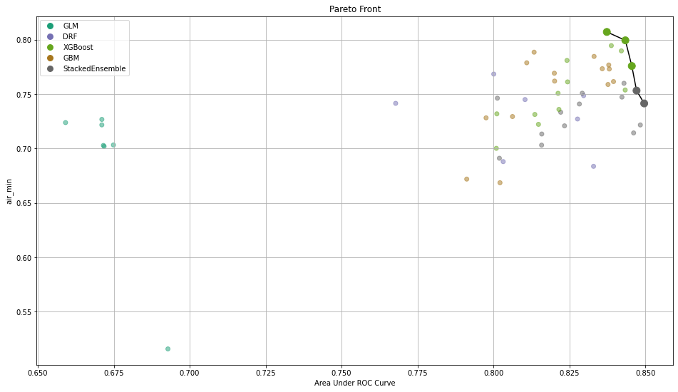
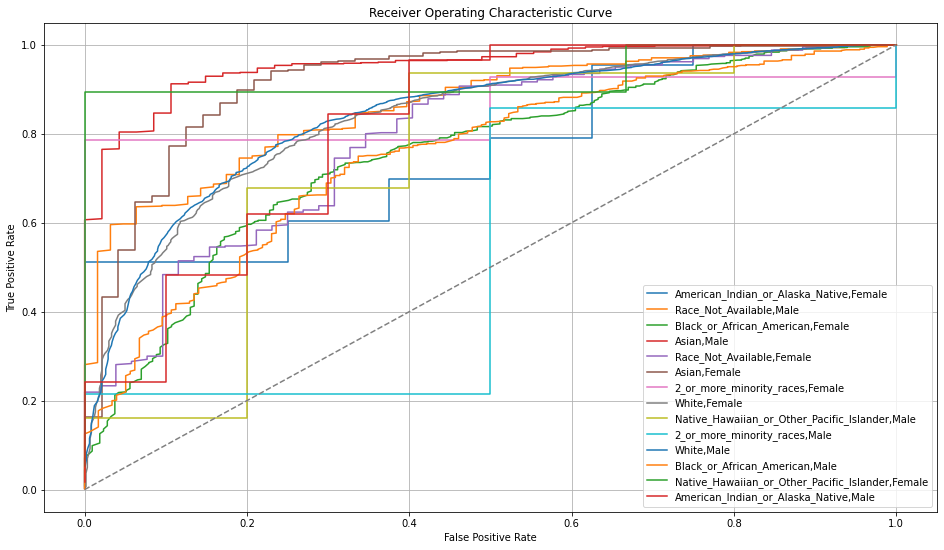
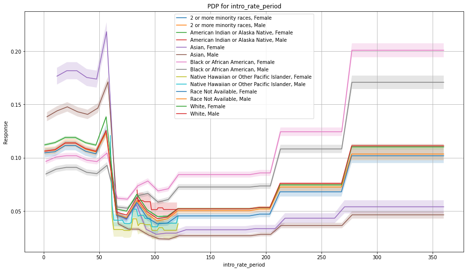
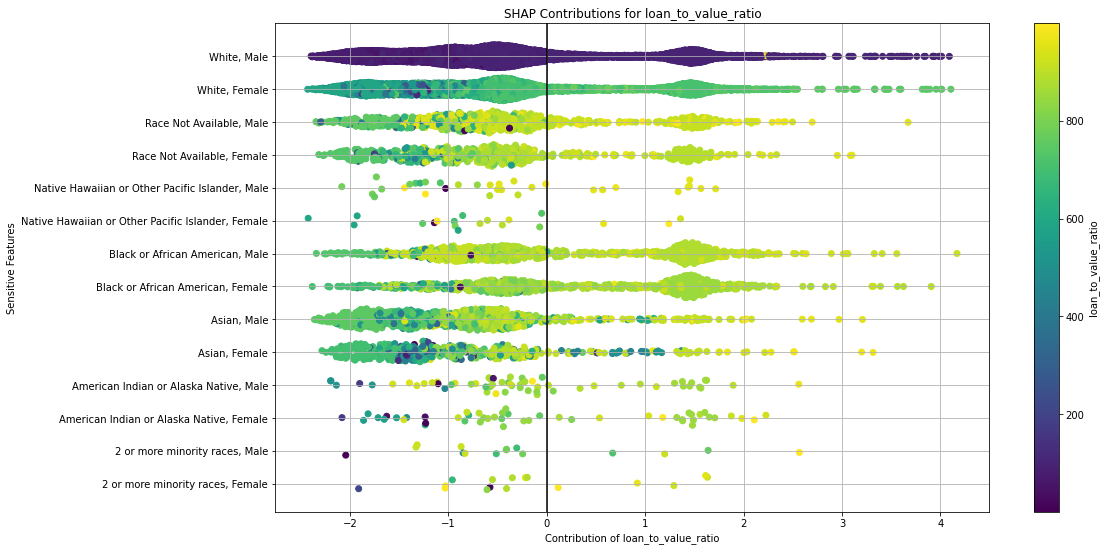
Once you pick a promising model, you can use <model_name>.inspect_model_fairness / h2o.inspect_model_fairness(<model_name>) to look at those metrics calculated on individual intersections. These include common performance metrics such as AUC, AUCPR, F1, etc., adverse impact ratio on those metrics, ROC, Precision-Recall Curve per intersection, PDP per intersection, and, if available (i.e. the model is a tree-based model), SHAP contributions per intersection. For more details, refer to the user guide.
Example
library(h2o)
h2o.init()

# Import the HDMA dataset:
f <- "https://erin-data.s3.amazonaws.com/admissible/data/hmda_lar_2018_sample.csv"
col_types <- list(by.col.name = c("high_priced"),
                  types = c("factor"))
df <- h2o.importFile(path = f, col.types = col_types)

# Split the data so you can compare the performance
# of admissible vs non-admissible models later:
splits <- h2o.splitFrame(df, ratios = 0.8, seed = 1)
train <- splits[[1]]
test <- splits[[2]]

# Set the response column and predictor columns:
y <- "high_priced"
x <- c("loan_amount",
       "loan_to_value_ratio",
       "loan_term",
       "intro_rate_period",
       "property_value",
       "income",
       "debt_to_income_ratio")

# Fairness related information:
protected_columns <- c("derived_race", "derived_sex")
reference <- c("White", "Male")
favorable_class <- "0"

# Train your models:
gbm1 <- h2o.gbm(x, y, train)
h2o.inspect_model_fairness(gbm1, test, protected_columns, reference, favorable_class)

# You will receive graphs with accompanying explanations in the terminal.
import h2o
from h2o.estimators import H2OGradientBoostingEstimator
h2o.init()

# Import the HDMA dataset:
f = "https://erin-data.s3.amazonaws.com/admissible/data/hmda_lar_2018_sample.csv"
col_types = {'high_priced': "enum"}
df = h2o.import_file(path=f, col_types=col_types)

# Split the data so you can compare the performance
# of admissible vs non-admissible models later:
train, test = df.split_frame(ratios=[0.8], seed=1)

# Set the response column and predictor columns:
y = "high_priced"
x =  ["loan_amount",
      "loan_to_value_ratio",
      "loan_term",
      "intro_rate_period",
      "property_value",
      "income",
      "debt_to_income_ratio"]

# Fairness related information:
protected_columns = ["derived_race", "derived_sex"]
reference = ["White", "Male"]
favorable_class = "0"

# Train your models:
gbm1 = H2OGradientBoostingEstimator()
gbm1.train(x, y, train)
gbm1.inspect_model_fairness(test, protected_columns, reference, favorable_class)

# You will receive graphs with accompanying explanations in the terminal.
Upgrade to XGBoost 1.6 (Adam Valenta)
The transition from XGBoost version 1.2 to 1.6 in the H2O-3 platform marks a major milestone in the evolution of this widely used algorithm. XGBoost, renowned for its efficiency and accuracy in handling structured datasets, has been a go-to choice for many data scientists. With the upgrade to version 1.6, H2O-3 raises the bar even further, providing users with an array of enhanced features and improvements.
One notable highlight of XGBoost 1.6 is its boosted performance, thanks to optimized algorithms and implementation. The upgrade includes various efficiency enhancements, such as improved parallelization strategies, memory management, and algorithmic tweaks. These improvements translate into faster training times and more efficient memory utilization, allowing you to process larger datasets and experiment with complex models more efficiently.
MOJO Support for H2OAssembly (Marek Novotný)
H2OAssembly is part of the H2O-3 API that enables you to form a pipeline of data munging operations. The new version of the class introduces the download_mojo method that converts an H2OAssembly pipeline to the MOJO2 artifact that is well-known from DriverlessAI. The conversion currently supports the following transformation stages:
H2OColSelect: selection of columnsH2OColOp: unary column operationsmath functions:
abs,acos,acosh,asin,asinh,atan,atanh,ceil,cos,cosh,cospi,digamma,exp,expm1,gamma,lgamma,log,log1p,log2,log10,logical_negation,sign,sin,sinh,sinpi,sqrt,tan,tanh,tanpi,trigamma,trunc,round,signifconversion functions:
ascharacter,asfactor,asnumeric,as_datestring functions:
lstrip,rstrip,gsub,sub,substring,tolower,toupper,trim,strsplit,countmatches,entropy,nchar,num_valid_substrings,greptime functions:
day,dayOfWeek,hour,minute,second,week,year
H2OBinaryOp: binary column operationsarithmetic functions:
__add__,__sub__,__mul__,__div__,__floordiv__,__pow__,__mod__comparison functions:
__le__,__lt__,__ge__,__gt__,__eq__,__ne__logical functions:
__and__,__or__string functions:
strdistance
Example
from h2o.assembly import *
from h2o.transforms.preprocessing import *

# Load the iris dataset:
iris = h2o.load_dataset("iris")

# Build your assembly:
assembly = H2OAssembly(steps=[("col_select",
                               H2OColSelect(["Sepal.Length",
                               "Petal.Length", "Species"])),
                              ("cos_Sepal.Length",
                               H2OColOp(op=H2OFrame.cos,
                               col="Sepal.Length", inplace=True)),
                              ("str_cnt_Species",
                               H2OColOp(op=H2OFrame.countmatches,
                               col="Species", inplace=False,
                               pattern="s"))])
result = assembly.fit(iris)

# Download the MOJO artifact:
assembly.download_mojo(file_name="iris_mojo", path='')
GBM Interpretability (Adam Valenta)
We brought another insight into H2O’s Gradient Boosting Machines (GBM) algorithm. This enhancement is the ability to retrieve row-to-tree assignments directly from the algorithm. This addresses the challenge of understanding how individual data points are assigned to specific decision trees within the ensemble. This new feature allows you to gain deeper insights into the decision-making process, thus enabling greater transparency and understanding of GBM models.
GBM Poisson Distribution Deviance (Yuliia Syzon)
Wehave updated the deviance calculation formula for the Poisson family in GBM. To ensure accurate and reliable results, we introduced a new formula:
which replaces the previously used formula:
This previous formula, though optimized and maintaining the deviance function behavior, produced incorrect output values. No longer! To validate the correctness of the new formula, we compared it with the deviance calculations in scikit-learn.
End of Support for Python 2.7 and 3.5 (Marek Novotný)
Support for Python 2.7 and 3.5 have been removed from the project to get rid of vulnerabilities connected with the future package. If you need to use Python 2.7 to 3.5, please contact sales@h2o.ai.
Documentation Improvements (Hannah Tillman)
Parameters for all supervised and unsupervised algorithms have been standardized, updated, reordered, and alphabetized to help you more easily find the information you need. Each section has been divvied up into algorithm-specific parameters and common parameters. GBM, DRF, XGBoost, Uplift DRF, Isolation Forest, and Extended Isolation Forest have an additional “shared tree-based algorithm parameters” section. All GLM family parameters have been centralized to the GLM page with icons showing which GLM family algorithm shares that parameter. Autoencoder for Deep Learning and HGLM for GLM also have their own parameter-specific sections.
The grid search hyperparameters have also been updated.
General Blogs
A Look at the UniformRobust method for histogram_type
Tree-based algorithms, especially Gradient Boosting Machines (GBM’s), are one of the most popular algorithms used. They often out-perform linear models and neural networks for tabular data since they used a boosted approach where each tree built works to fix the error of the previous tree. As the model trains, it is continuously self-correcting.
H2O-3’s GBM is able to train on real-world data out of the box: categoricals and missing values are automatically handled by the algorithm in a fully-distributed way. This means you can train the model on all your data without having to worry about sampling.
In this post, we talk about an improvement to how our GBM handles numeric columns. Traditionally, a GBM model would split numeric columns using uniform range-based splitting. Suppose you had a column that had values ranging from 0 to 100. It would split the column into bins 0-10, 11-20, 21-30, … 91-100. Each bin would be evaluated to determine the best way to split the data. The best split would be the one that most successfully splits your target column. For example, if you are trying to predict whether or not an employee will quit, the best split would be the one that could separate churn vs not-churn employees the most successfully.
However, when you’re handling data that has a column with outliers, this isn’t the most effective way to handle your data. Suppose you’re analyzing yearly income for a neighborhood: the vast majority of the people you’re looking at are making somewhere between $20-$80k. However, there are a few outliers in the neighborhood who make well-over $1 million. When splitting the column up for binning, it will still make uniform splits regardless of the distribution of data. Because the column splitting gets skewed with large outliers, all the outlier observations are classified into a single bin while the rest of the observations end up in another single bin. This, unfortunately, leaves most of the bins unused.
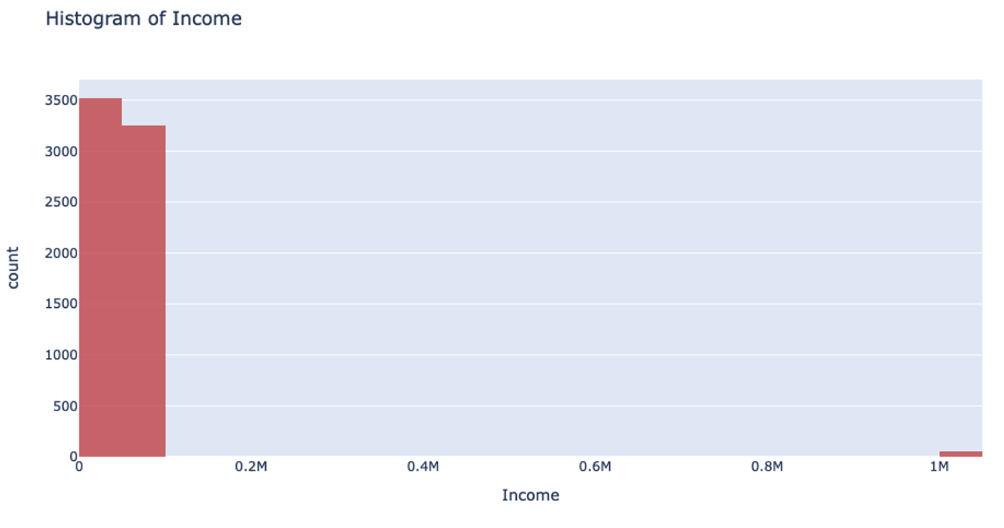
This can also drastically slow your prediction calculation since you’re iterating through so many empty bins. You also sacrifice accuracy because your data loses its diversity in this uneven binning method. Uniform splitting on data with outliers is full of issues.
The introduction of the UniformRobust method for histogram (histogram_type="UniformRobust") mitigates these issues! By learning from histograms from the previous layer, we are able to fine-tune the split points for the current layer.
The UniformRobust method isn’t impeded by outliers. It starts out using uniform range based binning. Then, it checks the distribution of the data in each bin. Many empty bins will indicate this range based binning is suboptimal, so it will iterate through all the bins and redefine them. If a bin contains no data, it’s deleted. If a bin contains too much data, then it’s split uniformly.
So, in the case that UniformRobust splitting fails (i.e. the distribution of values is still significantly skewed), the next iteration of finding splits attempts to correct the issue by repeating the procedure with new bins. This allows us to refine the promising bins recursively as we get deeper into the tree.
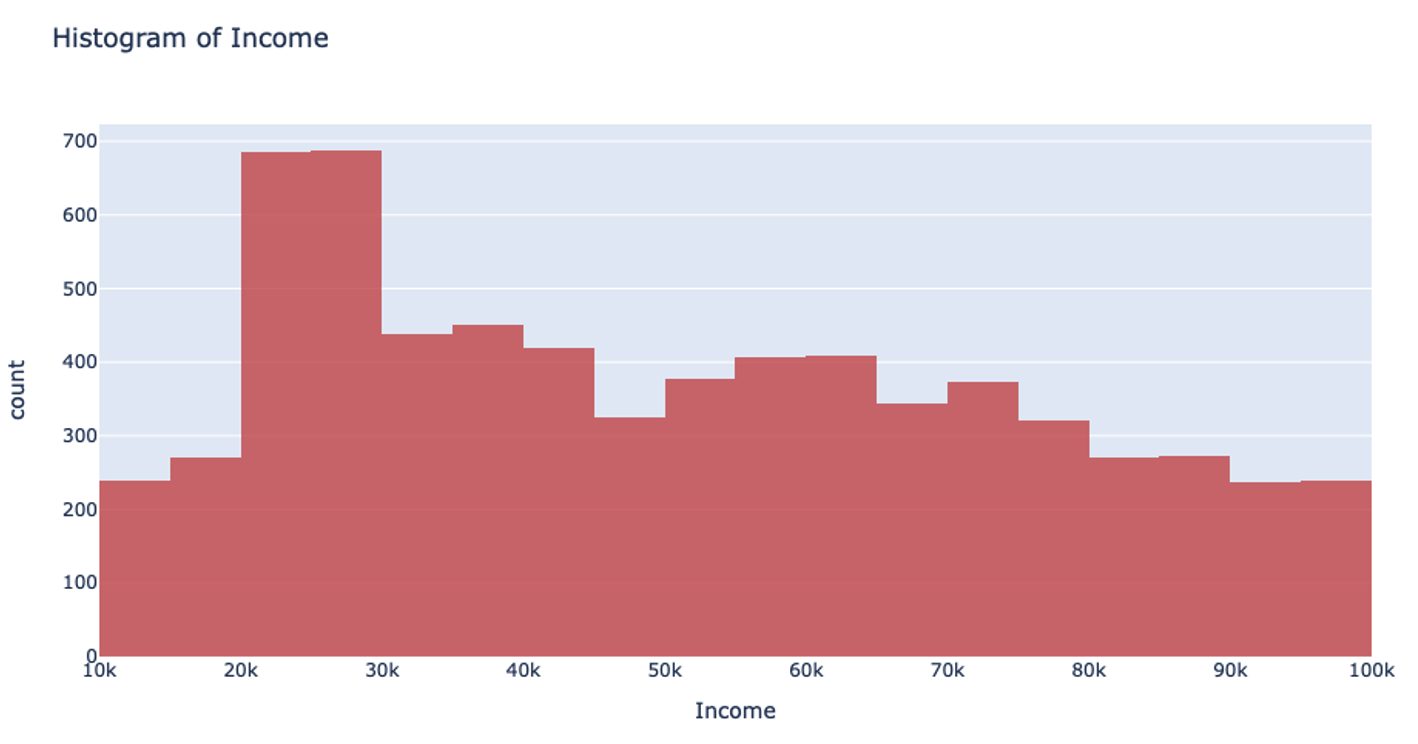
Let’s return to that income example. Using the UniformRobust method, we still begin with uniform splitting and see that very uneven distribution. However, what this method does next is to eliminate all those empty bins and split all the bins containing too much data. So, that bin that contained all the $0-100k yearly incomes is uniformly split. Then, with each iteration and each subsequent split, we will begin to see a much more even distribution of the data.
This method of splitting has the best available runtime performance and accuracy on datasets with outliers. We’re looking forward to you trying it out!
Example
In the following example, you can compare the performance of the UniformRobust method against the UniformAdaptive method on the Swedish motor insurance dataset. This dataset has slightly larger outliers in its Claims column.
library(h2o)
h2o.init()

# Import the Swedish motor insurance dataset. This dataset has larger outlier
# values in the "Claims" column:
motor <- h2o.importFile("http://h2o-public-test-data.s3.amazonaws.com/smalldata/glm_test/Motor_insurance_sweden.txt")

# Set the predictors and response:
predictors <- c("Payment", "Insured", "Kilometres", "Zone", "Bonus", "Make")
response <- "Claims"

# Build and train the UniformRobust model:
motor_robust <- h2o.gbm(histogram_type = "UniformRobust", seed = 1234, x = predictors, y = response, training_frame = motor)

# Build and train the UniformAdaptive model (we will use this model to
# compare with the UniformRobust model):
motor_adaptive <- h2o.gbm(histogram_type = "UniformAdaptive", seed = 1234, x = predictors, y = response, training_frame = motor)

# Compare the RMSE of the two models to see which model performed better:
print(c(h2o.rmse(motor_robust), h2o.rmse(motor_adaptive)))
[1] 36.03102 36.69582

# The RMSE is slightly lower in the UniformRobust model, showing that it performed better
# that UniformAdaptive on a dataset with outlier values!
import h2o
from h2o.estimators import H2OGradientBoostingEstimator
h2o.init()

# Import the Swedish motor insurance dataset. This dataset has larger outlier
# values in the "Claims" column:
motor = h2o.import_file("http://h2o-public-test-data.s3.amazonaws.com/smalldata/glm_test/Motor_insurance_sweden.txt")

# Set the predictors and response:
predictors = ["Payment", "Insured", "Kilometres", "Zone", "Bonus", "Make"]
response = "Claims"

# Build and train the UniformRobust model:
motor_robust = H2OGradientBoostingEstimator(histogram_type="UniformRobust", seed=1234)
motor_robust.train(x=predictors, y=response, training_frame=motor)

# Build and train the UniformAdaptive model (we will use this model to
# compare with the UniformRobust model):
motor_adaptive = H2OGradientBoostingEstimator(histogram_type="UniformAdaptive", seed=1234)
motor_adaptive.train(x=predictors, y=response, training_frame=motor)

# Compare the RMSE of the two models to see which model performed better:
print(motor_robust.rmse(), motor_adaptive.rmse())
36.03102136406947 36.69581743660738

# The RMSE is slightly lower in the UniformRobust model, showing that it performed better
# that UniformAdaptive on a dataset with outlier values!