Target Encoding
Target encoding is the process of replacing a categorical value with the mean of the target variable. In this example, we will be trying to predict bad_loan using our cleaned lending club data: https://raw.githubusercontent.com/h2oai/app-consumer-loan/master/data/loan.csv.
One of the predictors is addr_state, a categorical column with 50 unique values. To perform target encoding on addr_state, we will calculate the average of bad_loan per state (since bad_loan is binomial, this will translate to the proportion of records with bad_loan = 1).
For example, target encoding for addr_state could be:
| addr_state | average bad_loan |
|---|---|
| AK | 0.1476998 |
| AL | 0.2091603 |
| AR | 0.1920290 |
| AZ | 0.1740675 |
| CA | 0.1780015 |
| CO | 0.1433022 |
Instead of using state as a predictor in our model, we could use the target encoding of state.
In this topic, we will walk through the steps for using target encoding to convert categorical columns to numeric. This can help improve machine learning accuracy since algorithms tend to have a hard time dealing with high cardinality columns.
The jupyter notebook, categorical predictors with tree based model, discusses two methods for dealing with high cardinality columns:
- Comparing model performance after removing high cardinality columns
- Parameter tuning (specifically tuning
nbins_catsandcategorical_encoding)
In this topic, we will try using target encoding to improve our model performance.
Train Baseline Model
The examples below show how to train a baseline model.
library(h2o)
h2o.init()

# Start by training a model using the original data.
# Below we import our data into the H2O cluster.
df <- h2o.importFile("https://raw.githubusercontent.com/h2oai/app-consumer-loan/master/data/loan.csv")
df$bad_loan <- as.factor(df$bad_loan)

# Randomly split the data into 75% training and 25% testing.
# We will use the testing data to evaluate how well the model performs.
splits <- h2o.splitFrame(df, seed = 1234,
                         destination_frames=c("train.hex", "test.hex"),
                         ratios = 0.75)
train <- splits[[1]]
test <- splits[[2]]

# Now train the baseline model.
# We will train a GBM model with early stopping.
response <- "bad_loan"
predictors <- c("loan_amnt", "int_rate", "emp_length", "annual_inc", "dti",
                "delinq_2yrs", "revol_util", "total_acc", "longest_credit_length",
                "verification_status", "term", "purpose", "home_ownership",
                "addr_state")

gbm_baseline <- h2o.gbm(x = predictors, y = response,
                        training_frame = train, validation_frame = test,
                        score_tree_interval = 10, ntrees = 500,
                        sample_rate = 0.8, col_sample_rate = 0.8, seed = 1234,
                        stopping_rounds = 5, stopping_metric = "AUC",
                        stopping_tolerance = 0.001,
                        model_id = "gbm_baseline.hex")

# Get the AUC on the training and testing data:
train_auc <- h2o.auc(gbm_baseline, train = TRUE)
valid_auc <- h2o.auc(gbm_baseline, valid = TRUE)

auc_comparison <- data.frame('Data' = c("Training", "Validation"),
                             'AUC' = c(train_auc, valid_auc))

auc_comparison
        Data       AUC
1   Training 0.7492599
2 Validation 0.7070187
import h2o
h2o.init()

# Start by training a model using the original data.
# Below we import our data into the H2O cluster.
df = h2o.import_file("https://raw.githubusercontent.com/h2oai/app-consumer-loan/master/data/loan.csv")
df['bad_loan'] = df['bad_loan'].asfactor()

# Randomly split the data into 75% training and 25% testing.
# We will use the testing data to evaluate how well the model performs.
train, test = df.split_frame(ratios=[0.75], seed=1234)

# Now train the baseline model.
# We will train a GBM model with early stopping.
from h2o.estimators.gbm import H2OGradientBoostingEstimator
predictors = ["loan_amnt", "int_rate", "emp_length", "annual_inc", "dti",
              "delinq_2yrs", "revol_util", "total_acc", "longest_credit_length",
              "verification_status", "term", "purpose", "home_ownership",
              "addr_state"]
response = "bad_loan"

gbm_baseline=H2OGradientBoostingEstimator(score_tree_interval=10,
                                          ntrees=500,
                                          sample_rate=0.8,
                                          col_sample_rate=0.8,
                                          seed=1234,
                                          stopping_rounds=5,
                                          stopping_metric="AUC",
                                          stopping_tolerance=0.001,
                                          model_id="gbm_baseline.hex")

gbm_baseline.train(x=predictors, y=response, training_frame=train,
                   validation_frame=test)

# Get the AUC on the training and testing data:
train_auc = gbm_baseline.auc(train=True)
train_auc
0.7492599314713426

valid_auc = gbm_baseline.auc(valid=True)
valid_auc
0.707018686126265
Our training data has much higher AUC than our validation data. Review the Variable Importance values to see the variables with the greatest importance.
# Variable Importance
h2o.varimp_plot(gbm_baseline)
# Variable Importance
gbm_baseline.varimp_plot()
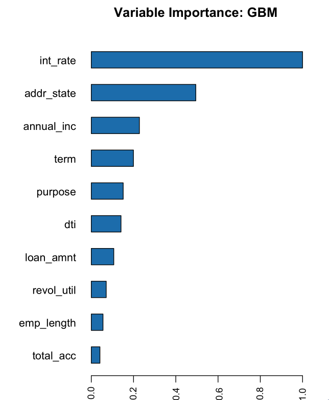
The variables with the greatest importance are int_rate, addr_state, annual_inc, and term. It makes sense that the int_rate has such high variable importance because this is related to loan default, but it is surprising that addr_state has such high variable importance. The high variable importance could be because our model is memorizing the training data through this high cardinality categorical column.
See if the AUC improves on the test data if we remove the addr_state predictor. This can indicate that the model is memorizing the training data.
predictors <- setdiff(predictors, "addr_state")

gbm_no_state <- h2o.gbm(x = predictors, y = response,
                        training_frame = train, validation_frame = test,
                        score_tree_interval = 10, ntrees = 500,
                        sample_rate = 0.8, col_sample_rate = 0.8, seed = 1234,
                        stopping_rounds = 5, stopping_metric = "AUC", stopping_tolerance = 0.001,
                        model_id = "gbm_no_state.hex")

# Get the AUC for the baseline model and the model without ``addr_state``
auc_baseline <- h2o.auc(gbm_baseline, valid = TRUE)
auc_nostate <- h2o.auc(gbm_no_state, valid = TRUE)

auc_comparison <- data.frame('Model' = c("Baseline", "No addr_state"),
                             'AUC' = c(auc_baseline, auc_nostate))

auc_comparison
          Model       AUC
1      Baseline 0.7070187
2 No addr_state 0.7076197
predictors = ["loan_amnt", "int_rate", "emp_length", "annual_inc", "dti",
              "delinq_2yrs", "revol_util", "total_acc", "longest_credit_length",
              "verification_status", "term", "purpose", "home_ownership"]

gbm_no_state=H2OGradientBoostingEstimator(score_tree_interval=10,
                                          ntrees=500,
                                          sample_rate=0.8,
                                          col_sample_rate=0.8,
                                          seed=1234,
                                          stopping_rounds=5,
                                          stopping_metric="AUC",
                                          stopping_tolerance=0.001,
                                          model_id="gbm_no_state.hex")

gbm_no_state.train(x=predictors, y=response, training_frame=train,
                   validation_frame=test)

auc_baseline = gbm_baseline.auc(valid=True)
auc_baseline
0.707018686126265

auc_nostate = gbm_no_state.auc(valid=True)
auc_nostate
0.7076197256885596
We see a slight improvement in our test AUC if we do not include the addr_state predictor. This is a good indication that the GBM model may be overfitting with this column.
Target Encoding in H2O-3
Now we will perform target encoding on addr_state to see if this representation improves our model performance.
Target encoding in H2O-3 is performed in two steps:
- Create (fit) a target encoding map using
target_encode_fit. This will contain the sum of the response column and the count. This can include an optionalfold_column. - Transform a target encoding map using
target_encode_transform. The target encoding map is applied to the data by adding new columns with the target encoding values.
The following options are available when performing target encoding, with some options preventing overfitting:
holdout_typeblended_avgnoisefold_columnsmoothinginflection_pointseed
Holdout Type
The holdout_type parameter defines whether the target average should be constructed on all rows of data. Overfitting can be prevented by removing some holdout data when calculating the target average on the training data.
The following holdout types can be specified:
none: no holdout. The mean is calculating on all rows of data **. This should be used for test dataloo: mean is calculating on all rows of data excluding the row itself.- This can be used for the training data. The target of the row itself is not included in the average to prevent overfitting.
kfold: The mean is calculating on out-of-fold data only. (This options requires a fold column.)- This can be used for the training data. The target average is calculated on the out of fold data to prevent overfitting
Blended Average
The blended_avg parameter defines whether the target average should be weighted based on the count of the group. It is often the case, that some groups may have a small number of records and the target average will be unreliable. To prevent this, the blended average takes a weighted average of the group’s target value and the global target value.
Noise
If random noise should be added to the target average, the noise parameter can be used to specify the amount of noise to be added. This value defaults to 0.01 * range of y of random noise.
Fold Column
Specify the name or column index of the fold column in the data. This defaults to NULL (no fold_column).
Smoothing
The smoothing value is used for blending and to calculate lambda. Smoothing controls the rate of transition between the particular level’s posterior probability and the prior probability. For smoothing values approaching infinity, it becomes a hard threshold between the posterior and the prior probability. This value defaults to 20.
Inflection Point
The inflection point value is used for blending and to calculate lambda. This determines half of the minimal sample size for which we completely trust the estimate based on the sample in the particular level of the categorical variable. This value defaults value to 10.
Seed
Specify a random seed used to generate draws from the uniform distribution for random noise. This defaults to -1.
Perform Target Encoding
Start by fitting the target encoding map. This has the number of bad loans per state (numerator) and the number of rows per state (denominator). After fitting the target encoding map, apply (transform) the target encoding per state.
Fit the Target Encoding Map
# Create a fold column in the train dataset
train$fold <- h2o.kfold_column(train, nfolds=5, seed = 1234)

# Fit the target encoding map
te_map <- h2o.target_encode_fit(train, x = list("addr_state"),
                                y = response, fold_column = "fold")
# Create a fold column in the train dataset
fold = train.kfold_column(n_folds=5, seed=1234)
fold.set_names(["fold"])
train = train.cbind(fold)

# Set the predictor to be "addr_state"
predictor = ["addr_state"]

# Fit the target encoding map
from h2o.targetencoder import TargetEncoder
target_encoder = TargetEncoder(x=predictor, y=response,
                               fold_column="fold",
                               blended_avg= True,
                               inflection_point = 3,
                               smoothing = 1,
                               seed=1234)
target_encoder.fit(train)
Transform Target Encoding
Apply the target encoding to our training and testing data.
Apply Target Encoding to Training Dataset
# Transform the target encoding on the training dataset
encoded_train <- h2o.target_encode_transform(train, x = list("addr_state"), y = response,
                                             target_encode_map = te_map, holdout_type = "kfold",
                                             fold_column="fold", blended_avg = TRUE,
                                             inflection_point=3, smoothing=1, seed = 1234,
                                             noise=0.2)
# noise = 0.2 will be applied
encoded_train = target_encoder.transform(frame=train, holdout_type="kfold", noise=0.2, seed=1234)
Apply Target Encoding to Testing Dataset
We do not need to apply any of the overfitting prevention techniques because our target encoding map was created on the training data, not the testing data.
holdout_type="none"blended_avg=FALSEnoise=0
encoded_test <- h2o.target_encode_transform(test, x = list("addr_state"), y = response,
                                            target_encode_map = te_map, holdout_type = "none",
                                            fold_column = "fold", noise = 0,
                                            blended_avg = FALSE, seed=1234)
target_encoder_test = TargetEncoder(x=predictor, y=response, blended_avg=False)
target_encoder_test.fit(train)

# Applying encoding map that was generated on `train` data to the `test`.
encoded_test = target_encoder_test.transform(frame=test, holdout_type="none", noise=0.0, seed=1234)
Train Model with KFold Target Encoding
Train a new model, this time replacing the addr_state with the addr_state_te.
predictors <- c("loan_amnt", "int_rate", "emp_length", "annual_inc",
                "dti", "delinq_2yrs", "revol_util", "total_acc",
                "longest_credit_length", "verification_status", "term",
                "purpose", "home_ownership", "addr_state_te")

gbm_state_te <- h2o.gbm(x = predictors,
                        y = response,
                        training_frame = encoded_train,
                        validation_frame = encoded_test,
                        score_tree_interval = 10,
                        ntrees = 500,
                        stopping_rounds = 5,
                        stopping_metric = "AUC",
                        stopping_tolerance = 0.001,
                        model_id = "gbm_state_te.hex",
                        seed=1234)
predictors = ["loan_amnt", "int_rate", "emp_length", "annual_inc",
              "dti", "delinq_2yrs", "revol_util", "total_acc",
              "longest_credit_length", "verification_status", "term",
              "purpose", "home_ownership", "addr_state_te"]

gbm_state_te = H2OGradientBoostingEstimator(score_tree_interval = 10,
                        ntrees = 500,
                        stopping_rounds = 5,
                        stopping_metric = "AUC",
                        stopping_tolerance = 0.001,
                        model_id = "gbm_state_te.hex",
                        seed=1234)
gbm_state_te.train(x=predictors, y=response,
                   training_frame=encoded_train,
                   validation_frame=encoded_test)
The AUC three models are shown below:
# Get AUC
auc_state_te <- h2o.auc(gbm_state_te, valid = TRUE)

auc_comparison <- data.frame('Model' = c("No Target Encoding",
                                         "No addr_state",
                                         "addr_state Target Encoding"),
                             'AUC' = c(auc_baseline, auc_nostate, auc_state_te))

auc_comparison
                       Model       AUC
1         No Target Encoding 0.7070187
2              No addr_state 0.7076197
3 addr_state Target Encoding 0.7072750
# Compare AUC values:

valid_auc = gbm_baseline.auc(valid=True)
valid_auc
0.707018686126265

auc_nostate = gbm_no_state.auc(valid=True)
auc_nostate
0.7076197256885596

auc_state_te = gbm_state_te.auc(valid=True)
auc_state_te
0.7072749724799465
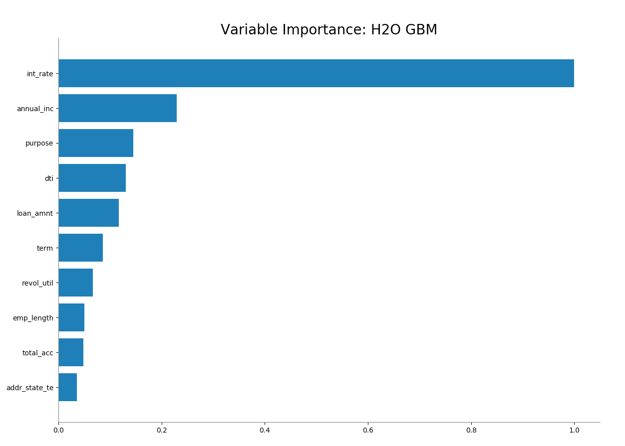
Now the addr_state_te has much smaller variable importance. It is no longer the second most important feature but the 10th.
# Variable Importance
h2o.varimp_plot(gbm_state_te)
# Variable Importance
gbm_state_te.varimp_plot()
References
- Target Encoding in H2O-3 Demo
- Automatic Feature Engineering Webinar
- Daniele Micci-Barreca. 2001. A preprocessing scheme for high-cardinality categorical attributes in classification and prediction problems. SIGKDD Explor. Newsl. 3, 1 (July 2001), 27-32.