H2O-3 Major Release Blogs
H2O Release 3.36 (Zorn)

There’s a new major release of H2O, and it’s packed with new features and fixes! This release includes the official support of Java 17, the ability to import GAM MOJO models, and the ability to import old MOJO models into newer versions of H2O. Read about all of Rel-Zorn’s new features and fixes here.
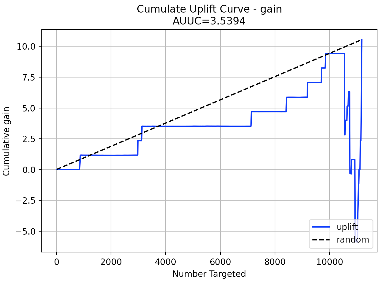
Distributed Uplift Random Forest
Distributed Uplift Random Forest (Uplift DRF) is a classification tool for modeling uplift: the incremental impact of a treatment. This tool is very useful in marketing and medicine, and this machine learning approach is inspired by the A/B testing method.
Demo
Here is a Jupyter notebook where H2O Uplift DRF is compared to implementation Uplift RF from CausalML library.
Example
library(h2o)
h2o.init()

# Import the uplift dataset into H2O:
data <- h2o.importFile("https://s3.amazonaws.com/h2o-public-test-data/smalldata/uplift/criteo_uplift_13k.csv")

# Set the predictors, response, and treatment column:
# set the predictors
predictors <- c("f1", "f2", "f3", "f4", "f5", "f6","f7", "f8")
# set the response as a factor
data$conversion <- as.factor(data$conversion)
# set the treatment column as a factor
data$treatment <- as.factor(data$treatment)

# Split the dataset into a train and valid set:
data_split <- h2o.splitFrame(data = data, ratios = 0.8, seed = 1234)
train <- data_split[[1]]
valid <- data_split[[2]]

# Build and train the model:
uplift.model <- h2o.upliftRandomForest(training_frame = train,
                                       validation_frame=valid,
                                       x=predictors,
                                       y="conversion",
                                       ntrees=10,
                                       max_depth=5,
                                       treatment_column="treatment",
                                       uplift_metric="KL",
                                       min_rows=10,
                                       seed=1234,
                                       auuc_type="qini")
# Eval performance:
perf <- h2o.performance(uplift.model)

# Generate predictions on a validation set (if necessary)
predict <- h2o.predict(uplift.model, newdata = valid)

# Plot Uplift Curve
plot(perf, metric="gain")
import h2o
from h2o.estimators import H2OUpliftRandomForestEstimator
h2o.init()

# Import the cars dataset into H2O:
data = h2o.import_file("https://s3.amazonaws.com/h2o-public-test-data/smalldata/uplift/criteo_uplift_13k.csv")

# Set the predictors, response, and treatment column:
predictors = ["f1", "f2", "f3", "f4", "f5", "f6","f7", "f8"]
# set the response as a factor
response = "conversion"
data[response] = data[response].asfactor()
# set the treatment as a factor
treatment_column = "treatment"
data[treatment_column] = data[treatment_column].asfactor()

# Split the dataset into a train and valid set:
train, valid = data.split_frame(ratios=[.8], seed=1234)

# Build and train the model:
uplift_model = H2OUpliftRandomForestEstimator(ntrees=10,
                                              max_depth=5,
                                              treatment_column=treatment_column,
                                              uplift_metric="KL",
                                              min_rows=10,
                                              seed=1234,
                                              auuc_type="qini")
uplift_model.train(x=predictors,
                   y=response,
                   training_frame=train,
                   validation_frame=valid)

# Eval performance:
perf = uplift_model.model_performance()

# Generate predictions on a validation set (if necessary)
pred = uplift_model.predict(valid)

# Plot Uplift curve from performance
perf.plot_uplift(metric="gain", plot=True)
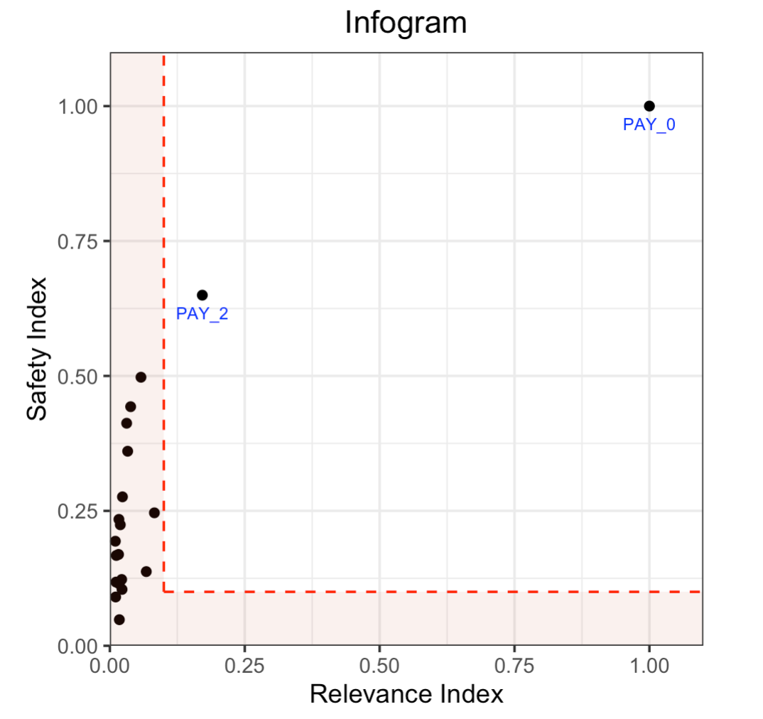
Infogram & Admissible Machine Learning
The Infogram reduces bias in built models by taking protected variables (e.g., race and gender) into account. It does this by measuring the admissibility of a variable. This is determined by a safety and relevancy index which serves as a diagnostic tool for fairness. When variables are determined to be unsafe, they will be considered inadmissible.
Example
library(h2o)

h2o.init()

# Import credit dataset
f <- "https://erin-data.s3.amazonaws.com/admissible/data/taiwan_credit_card_uci.csv"
col_types <- list(by.col.name = c("SEX", "MARRIAGE", "default_payment_next_month"),
                  types = c("factor", "factor", "factor"))
df <- h2o.importFile(path = f, col.types = col_types)

# We will split the data so that we can test/compare performance
# of admissible vs non-admissible models later
splits <- h2o.splitFrame(df, seed = 1)
train <- splits[[1]]
test <- splits[[2]]

# Response column and predictor columns
y <- "default_payment_next_month"
x <- setdiff(names(train), y)

# Protected columns
pcols <- c("SEX", "MARRIAGE", "AGE")

# Infogram
ig <- h2o.infogram(y = y, x = x, training_frame = train, protected_columns = pcols)
plot(ig)

# Admissible score frame
asf <- ig@admissible_score
asf
import h2o
from h2o.estimators.infogram import H2OInfogram

h2o.init()

# Import credit dataset
f = "https://erin-data.s3.amazonaws.com/admissible/data/taiwan_credit_card_uci.csv"
col_types = {'SEX': "enum", 'MARRIAGE': "enum", 'default_payment_next_month': "enum"}
df = h2o.import_file(path=f, col_types=col_types)

# We will split the data so that we can test/compare performance
# of admissible vs non-admissible models later
train, test = df.split_frame(seed=1)

# Response column and predictor columns
y = "default_payment_next_month"
x = train.columns
x.remove(y)

# Protected columns
pcols = ["SEX", "MARRIAGE", "AGE"]

# Infogram
ig = H2OInfogram(protected_columns=pcols)
ig.train(y=y, x=x, training_frame=train)
ig.plot()

# Admissible score frame
asf = ig.get_admissible_score_frame()
asf
Model Selection
Model Selection will help you select the best predictor subsets from your dataset when building GLM regression models.
Example
library(h2o)
h2o.init()

# Import the prostate dataset:
prostate <- h2o.importFile("http://s3.amazonaws.com/h2o-public-test-data/smalldata/logreg/prostate.csv")

# Set the predictors & response:
predictors <- c("AGE", "RACE", "CAPSULE", "DCAPS", "PSA", "VOL", "DPROS")
response <- "GLEASON"

# Build & train the model:
allsubsetsModel <- h2o.modelSelection(x = predictors,
                                      y = response,
                                      training_frame = prostate,
                                      seed = 12345,
                                      max_predictor_number = 7,
                                      mode = "allsubsets")

# Retrieve the results (H2OFrame containing best model_ids, best_r2_value, & predictor subsets):
results <- h2o.result(allsubsetsModel)
print(results)
import h2o
from h2o.estimators import H2OModelSelectionEstimator
h2o.init()

# Import the prostate dataset:
prostate = h2o.import_file("http://s3.amazonaws.com/h2o-public-test-data/smalldata/logreg/prostate.csv")

# Set the predictors & response:
predictors = ["AGE","RACE","CAPSULE","DCAPS","PSA","VOL","DPROS"]
response = "GLEASON"

# Build & train the model:
maxrModel = H2OModelSelectionEstimator(max_predictor_number=7,
                                       seed=12345,
                                       mode="maxr")
maxrModel.train(x=predictors, y=response, training_frame=prostate)

# Retrieve the results (H2OFrame containing best model_ids, best_r2_value, & predictor subsets):
results = maxrModel.result()
print(results)
RuleFit Improvements
For RuleFit, the new h2o.predict_rules() method evaluates the validity of given rules on the given data. The lambda parameter, specified during model building, has also been exposed giving you better control over the regularization strength.
Example
# Import the titanic dataset and set the column types:
f <- "https://s3.amazonaws.com/h2o-public-test-data/smalldata/gbm_test/titanic.csv"
coltypes <- list(by.col.name = c("pclass", "survived"), types=c("Enum", "Enum"))
df <- h2o.importFile(f, col.types = coltypes)

# Split the dataset into train and test:
splits <- h2o.splitFrame(data = df, ratios = 0.8, seed = 1)
train <- splits[[1]]
test <- splits[[2]]

# Set the predictors and response:
response <- "survived"
predictors <- c("age", "sibsp", "parch", "fare", "sex", "pclass")

# Build and train the model:
rfit <- h2o.rulefit(y = response,
                    x = predictors,
                    training_frame = train,
                    max_rule_length = 10,
                    max_num_rules = 100,
                    seed = 1)

# Retrieve the rule importance:
print(rfit@model$rule_importance)

# Choose a rule id and check its validity (for example, "M0T49N14" & "M0T9N17"):
h2o.predict_rules(rfit, train, c("M0T49N14", "M0T9N17"))
from h2o.estimators import H2ORuleFitEstimator

# Import the titanic dataset and set the column types:
f = "https://s3.amazonaws.com/h2o-public-test-data/smalldata/gbm_test/titanic.csv"
df = h2o.import_file(path=f, col_types={'pclass': "enum", 'survived': "enum"})

# Split the dataset into train and test:
train, test = df.split_frame(ratios=[0.8], seed=1)

# Set the predictors and response:
x = ["age", "sibsp", "parch", "fare", "sex", "pclass"]
y = "survived"

# Build and train the model:
rfit = H2ORuleFitEstimator(max_rule_length=10,
                           max_num_rules=100,
                           seed=1)
rfit.train(training_frame=train, x=x, y=y)

# Retrieve the rule importance:
print(rfit.rule_importance())

# Choose a rule id and check its validity (for example, "M0T49N14" & "M0T9N17"):
rfit.predict_rules(train, ['M0T49N14','M0T9N17'])
AutoML Improvements
Under resource-constrained environments, AutoML’s validation and stacking strategy has updated to speed up processing: with datasets that are large in comparison to their available computation resources, we shifted to a blending strategy using holdout frames (this is an automated version of using the blending_frame argument). We have also improved error handling: your AutoML model will detect and fail earlier when there are problems with your data. This allows you to debug more quickly.