Gradient Boosted Regression and Classification
Gradient Boosted Regression and Gradient Boosted Classification are forward learning ensemble methods. The guiding heuristic is that good predictive results can be obtained through increasingly refined approximations.
Defining a GBM Model
Destination Key:
A user defined name for the model.
Source:
The .hex key associated with the parsed data to be used in the model.
Response:
The dependent variable to be modeled. Dependent variables can be binomial indicators, multinomial classes (if the classes are
Ignored Columns:
By default all of the information submitted in a data set will be used in building the GBM model. Users specify those attributes that should be omitted from analysis by highlighting them.
Classification:
An option that treats the outcome variable as categorical, and when unchecked treats the outcome variable as continuous. If a continuous real variable has been defined for the response, H2O will return an error if a classification model is requested.
Validation:
A .hex key associated with data to be used in validation of the model built using the data specified in Source.
NTrees:
The number of trees to be built. Models with different total numbers of trees can be specified by entering the different values as a comma separated list. For example,to specify different models with 200, 100 and 50 trees respectively enter “200, 100, 50”.
Max Depth:
The maximum number of edges to be generated between the first node and the terminal node. To test different depths, values can be specified in a comma separated list.
Min Rows:
The minimum number of observations to be included in a terminal leaf. If any classification must consist of no fewer than five elements, min rows should be set to five.
NBins:
The number of bins data are partitioned into before the best split point is determined. A high number of bins relative to a low number of observations will have a small number of observations in each bin. As the number of bins approaches the number of unique values in a column, the analysis approaches evaluation of all possible split points
Score Each Iteration:
An option that returns error rate information after each tree in the requested set is built. This option allows users to evaluate the marginal gain in fit from building that tree, allowing for interruption of the model when the gain for building the next tree isn’t substantial enough to continue building. Users should be aware that this option can slow the model building process, depending on the size and shape of both the training data and the testing data.
Importance:
An option that returns information about each variable’s importance in training the specified model.
Learn Rate:
A number between 0 and 1 that specifies the rate at which the algorithm should converge. Learning rate is inversely related to the number of iterations taken for the algorithm to complete.
Grid Parallelism:
When multiple models are called for through the grid search options such as specification of multiple learning rates, selecting this option will build the set of models in parallel rather than sequentially.
Treatment of Factors
When the specified GBM model includes factors, those factors are analyzed by assigning each distinct factor level an integer, and then binning the ordered integers according to the user specified number of bins (N Bins). Split points are determined by considering as the end points of each bin, and the one versus many split for each bin.
For example, if the factor is split into 5 bins, H2O orders the bins by bin number, and then the split between the first and second bin, the second and third, the third and fourth, and the fourth and fifth are considered. Additionally the split that comes of splitting the first bin from the other four, and all analogous splits for the other four bins are considered. If users wish to specify a model such that all factors are considered individually, they can do so by setting N Bins equal to the number of factor levels. This can be done even in excess of 1024 levels (the maximum number of levels that can be handled in R), though this will increase the time it takes for a model to be fully generated.
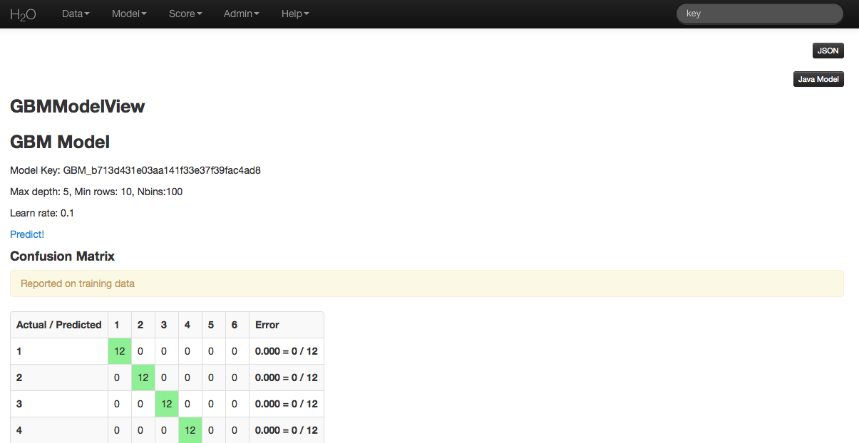
Interpreting Results
GBM results for classification models are comprised of a confusion matrix and the mean squared error of each tree. Note that when MSE for each tree is returned, the first and second MSE values are the same. The initial MSE is calculated for the dependent variable, and is given as a baseline against which to evaluate the predictive performance of each next basis function. The first MSE value given is the MSE for the data set before any trees are built.
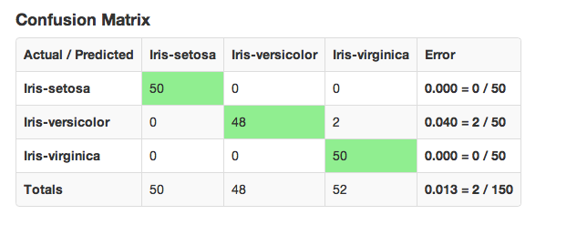
An example of a confusion matrix is given below:
The highlighted fields across the diagonal indicate the number the number of true members of the class who were correctly predicted as true. The overall error rate is shown in the bottom right field. It reflects the proportion of incorrect predictions overall.
For regression models, returned results MSE
Mean squared error is an indicator of goodness of fit. It measures the squared distance between an estimator and the estimated parameter.
Cost of Computation
The cost of computation in GBM is bounded above in the following way:
\(Cost = bins\times (2^{leaves}) \times columns \times classes\)
GBM Algorithm
H2O’s Gradient Boosting Algorithms follow the algorithm specified by Hastie et al (2001):
Initialize \(f_{k0} = 0,\: k=1,2,…,K\)
- \(For\:m=1\:to\:M:\)
\((a)\:Set\:\) \(p_{k}(x)=\frac{e^{f_{k}(x)}}{\sum_{l=1}^{K}e^{f_{l}(x)}},\:k=1,2,…,K\)
\((b)\:For\:k=1\:to\:K:\)
\(\:i.\:Compute\:r_{ikm}=y_{ik}-p_{k}(x_{i}),\:i=1,2,…,N.\)
\(\:ii.\:Fit\:a\:regression\:tree\:to\:the\:targets\:r_{ikm},\:i=1,2,…,N\)
\(giving\:terminal\:regions\:R_{jim},\:j=1,2,…,J_{m}.\)
\(\:iii.\:Compute\)
\(\gamma_{jkm}=\frac{K-1}{K}\:\frac{\sum_{x_{i}\in R_{jkm}}(r_{ikm})}{\sum_{x_{i}\in R_{jkm}}|r_{ikm}|(1-|r_{ikm})},\:j=1,2,…,J_{m}.\)\(\:iv.\:Update\:f_{km}(x)=f_{k,m-1}(x)+\sum_{j=1}^{J_{m}}\gamma_{jkm}I(x\in\:R_{jkm}).\)
Output \(\:\hat{f_{k}}(x)=f_{kM}(x),\:k=1,2,…,K.\)
BETA: Standalone Scoring:
As a beta feature still undergoing testing, GBM models now offer users an option to download a generated GBM model in java code. This new feature can be accessed by clicking Java Model in the upper right corner. When the model is small enough, the java code for the model will be made available to inspect from within the GUI, larger models can be inspected after users have downloaded the model.
To download the model open the terminal window, create a directory where the model will be saved, set the new directory as the working directory and follow the curl and java compile commands displayed in the instructions at the top of the java model.
Reference
Dietterich, Thomas G, and Eun Bae Kong. “Machine Learning Bias, Statistical Bias, and Statistical Variance of Decision Tree Algorithms.” ML-95 255 (1995).
Elith, Jane, John R Leathwick, and Trevor Hastie. “A Working Guide to Boosted Regression Trees.” Journal of Animal Ecology 77.4 (2008): 802-813
Friedman, Jerome H. “Greedy Function Approximation: A Gradient Boosting Machine.” Annals of Statistics (2001): 1189-1232.
Friedman, Jerome, Trevor Hastie, Saharon Rosset, Robert Tibshirani, and Ji Zhu. “Discussion of Boosting Papers.” Ann. Statist 32 (2004): 102-107
Friedman, Jerome, Trevor Hastie, and Robert Tibshirani. “Additive Logistic Regression: A Statistical View of Boosting (With Discussion and a Rejoinder by the Authors).” The Annals of Statistics 28.2 (2000): 337-407 http://projecteuclid.org/DPubS?service=UI&version=1.0&verb=Display&handle=euclid.aos/1016218223
Hastie, Trevor, Robert Tibshirani, and J Jerome H Friedman. The Elements of Statistical Learning. Vol.1. N.p., page 339: Springer New York, 2001. http://www.stanford.edu/~hastie/local.ftp/Springer/OLD//ESLII_print4.pdf
Niu, Feng, et al. “Hogwild!: A lock-free approach to parallelizing stochastic gradient descent.” Advances in Neural Information Processing Systems 24 (2011): 693-701. (algorithm implemented is on p.5) https://papers.nips.cc/paper/4390-hogwild-a-lock-free-approach-to-parallelizing-stochastic-gradient-descent.pdf