GBM Tutorial
This tutorial walks the new user through a GBM analysis in H2O.
If you have never used H2O before, refer to the quick start guide for additional instructions on how to run H2O Getting Started From a Downloaded Zip File.
Getting Started
This tutorial uses a publicly available data set that can be found at: http://archive.ics.uci.edu/ml/datasets/Arrhythmia
The original data are the Arrhythmia data set made available by UCI Machine Learning repository. They are composed of 452 observations and 279 attributes.
Before modeling, parse data into H2O:
- From the drop-down Data menu, select Upload and use the uploader to upload data.
- On the “Request Parse” page that appears, check the “header” checkbox if the first row of the data set is a header. No other changes are required.
- Click Submit. Parsing data into H2O generates a .hex key in the format “data name.hex”

Building a Model
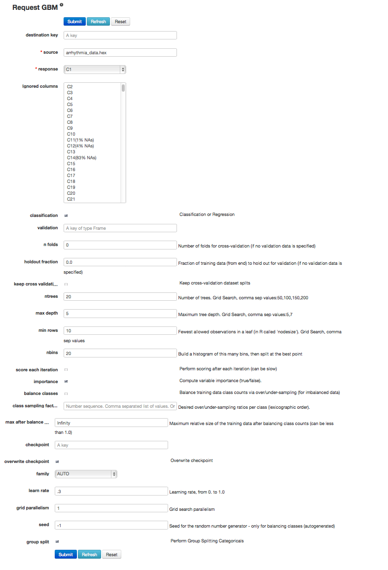
- Once data are parsed, a horizontal menu displays at the top of the screen reading “Build model using ... ”. Select Distributed GBM here, or go to the drop down menu Model and select Gradient Boosting Machine.
- In the “source” field, enter the .hex key for the Arrhythmia data set, if it is not already entered.
- From the drop-down “response” list, select C1.
- Select Gradient Boosted Classification by checking the “classification” checkbox or Gradient Boosted Regression by unchecking the “classification” checkbox. GBM is set to classification by default. For this example, check the classification checkbox.
- In the “ntrees” field, enter the number of trees to generate. For this example, enter 20.
- In the “max depth” field, specify the maximum number of edges between the top node and the furthest node as a stopping criteria. For this example, enter 5.
- In the “min rows” field, specify the minimum number of observations (rows) to include in any terminal node as a stopping criteria. For this example, use 25.
- In the “nbins” field, specify the number of bins to use for splitting data. For this example, use the default value of 20. Split points are evaluated at the boundaries of each of these bins. As the value for Nbins increases, the more closely the algorithm approximates evaluating each individual observation as a split point. The trade off for this refinement is an increase in computational time.
- In the “learn rate” field, specify a value to slow the convergence of the algorithm to a solution and help prevent overfitting. This parameter is also referred to as shrinkage. For this example, enter .3.
- To generate the model, click the Submit button.
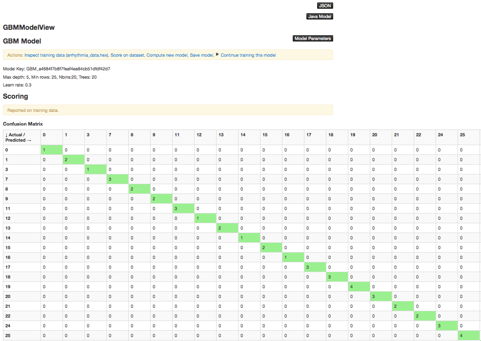
GBM Results
The GBM output for classification displays a confusion matrix with the classifications for each group, the associated error by group, and the overall average error. Regression models can be quite complex and difficult to directly interpret. For that reason, H2O provides a model key for subsequent use in validation and prediction.
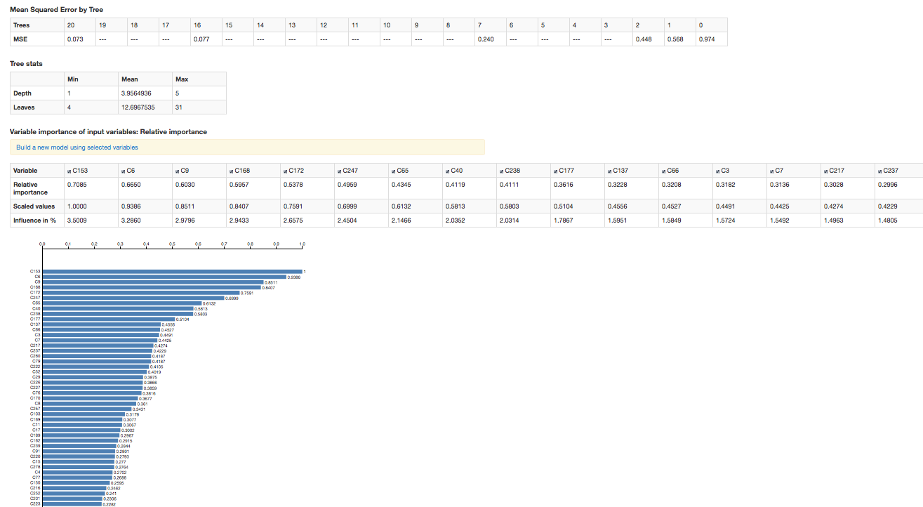
- Both model types provide the MSE by tree.
- For classification models, the MSE is based on the classification error within the tree.
- For regression models, MSE is calculated from the squared deviances, as with standard regressions.
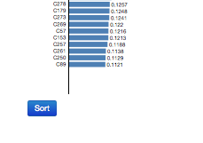
The output also includes a table containing the tree statistics (min, max, and mean for tree depth and number of leaves), as well as a table and chart representing the variable importances.
To change the order in which the variable importances are displayed (from most important to least or vice versa), click the Sort button below the chart.