GLM Grid Tutorial
This tutorial walks the new user through a GLM grid analysis, describing how to specify, run, and interpret a GLM grid model using H2O. Specification of GLM grid models is similar to creating GLM models, and all parameters and results have the same meaning. The primary difference between GLM and GLM Grid is that you can specify several different models and generate the specified models simultaneously. For more information, refer to the GLM tutorial GLM Tutorial
If you have never used H2O before, refer to the quick start guide for additional instructions on how to run H2O Getting Started From a Downloaded Zip File
When to Use GLM Grid
Use GLM Grid if the variable of interest relates to predictions or inferences about a rate, an event, or a continuous measurement, or to answer questions about how a set of environmental conditions influence the dependent variable when the error rates in prediction are likely to be sensitive to the degree of regularization applied, or specified thresholds.
Here are some examples:
- What attributes determine which customers will purchase, and which will not?
- Given a set of specific manufacturing conditions, how many units produced will fail?
- How many customers will contact help support in a given time frame?
- Given a set of conditions, which units will fail?
Getting Started
This tutorial uses a publicly-available data set that can be found at:
http://archive.ics.uci.edu/ml/machine-learning-databases/abalone/
The original data are the Abalone data set made available by UCI Machine Learning repository. They are composed of 4177 observations of 9 attributes. All attributes are real valued continuous, except for Sex and Rings (found in columns 0 and 8 respectively). Sex is categorical with 3 levels (male, female, and infant), and Rings is integer-valued.
Before modeling, parse data into H2O as follows:
- From the drop-down Data menu, select Upload, and use the uploader to upload data.
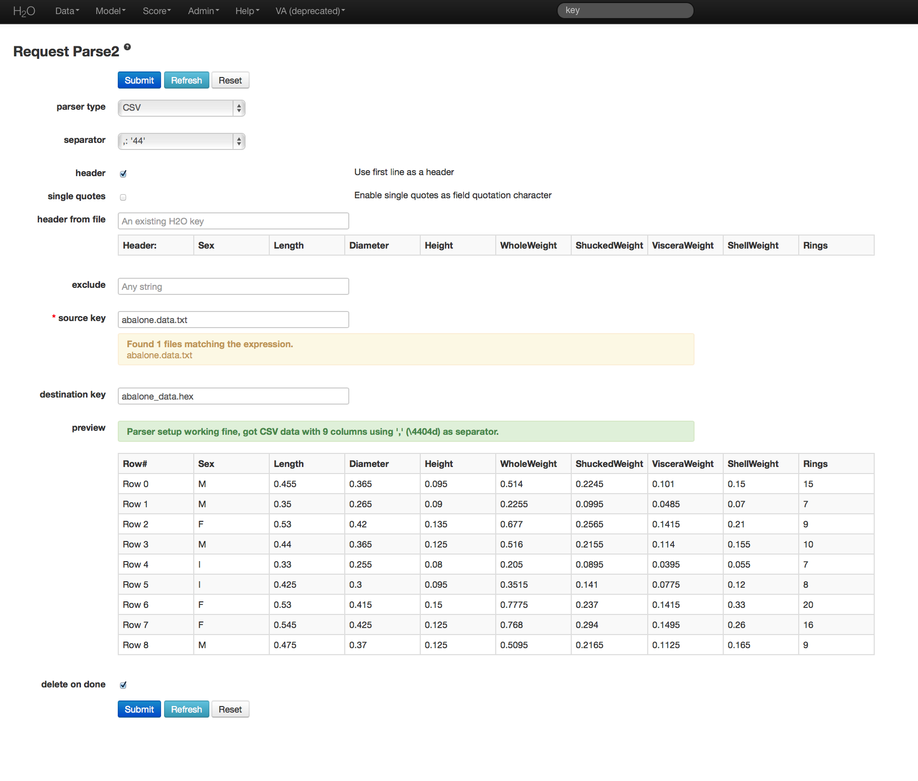
- On the “Request Parse” page that appears, check the “header” checkbox if the first row of the data set is a header. No other changes are required.
- Click Submit. Parsing data into H2O generates a .hex key of the form “data name.hex”
Building a Model
- Once data are parsed, a horizontal menu appears at the top of the screen reading “Build model using ... ”. Select Generalized Linear Model, or go to the drop down menu Model and select GLM.
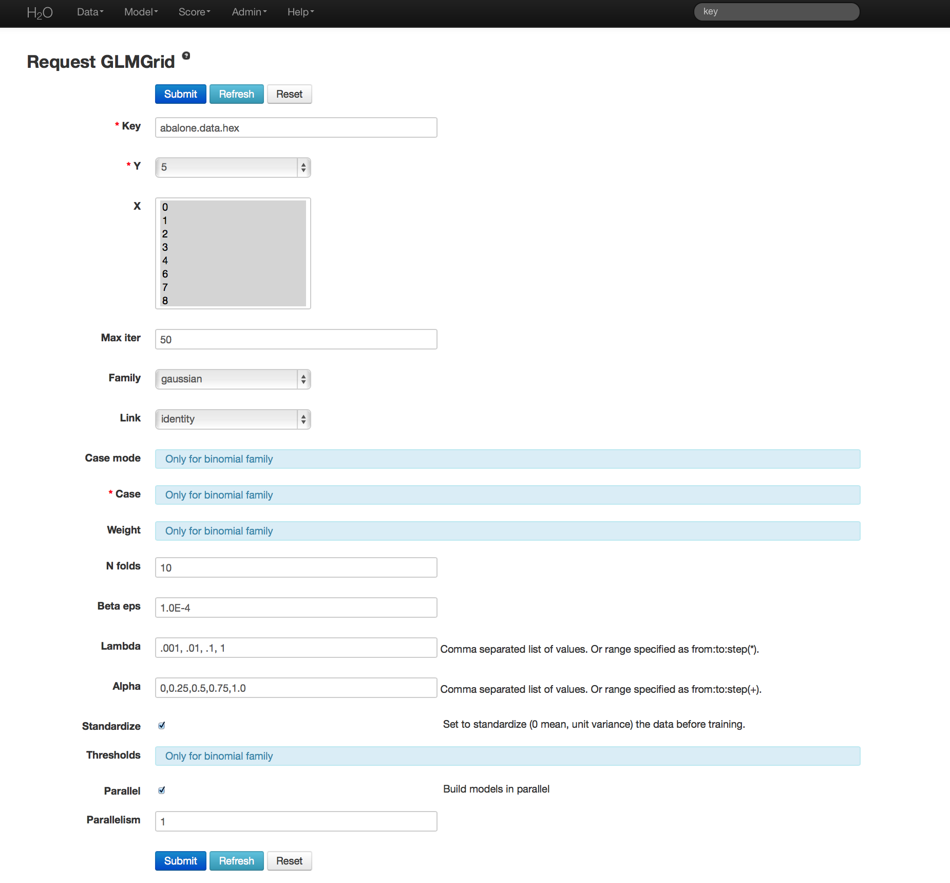
- In the “source” field, enter the .hex key for the data set.
- From the drop-down “response” list, select the column associated with the Whole Weight variable (column 5).
- In the “Ignored Columns” area, select the columns associated with Sex, Length, Diameter, Height, and Rings (all other columns).
- Select “gaussian” from the drop-down “family” list.
- “Lambda” and “alpha” are the parameters that determine the regularization of GLM models. To find detailed information on the specification of tuning parameters, refer to the data science documentation on GLM Generalized Linear Model. In GLM Grid specification, specify a range of values by entering the values as a comma-separated list (for example: 0.001, 0.01, 0.1, 1 will produce models at each of the four specified levels). The same syntax holds for alpha and threshold specification.
- Confirm the value for “n-folds” is 10. This will produce 10 cross-validation models for each unique combination of the specified parameters.
- Confirm that the “standardization” checkbox is checked. This option displays two sets of coefficients: the non-standardized coefficients and the standardized coefficients.
GLM Grid Results
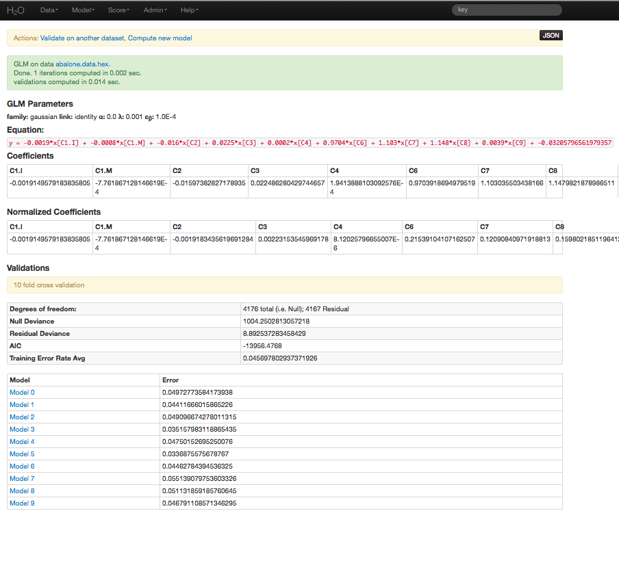
The GLM grid output includes a table of the specified models, along with each model’s corresponding specification values. View individual models by clicking the active link for each model. The AIC and error rate display for each model’s coefficients (as well as normalized coefficients when standardization is enabled). An equation of the specified model displays in red at the top of the GLM results page.
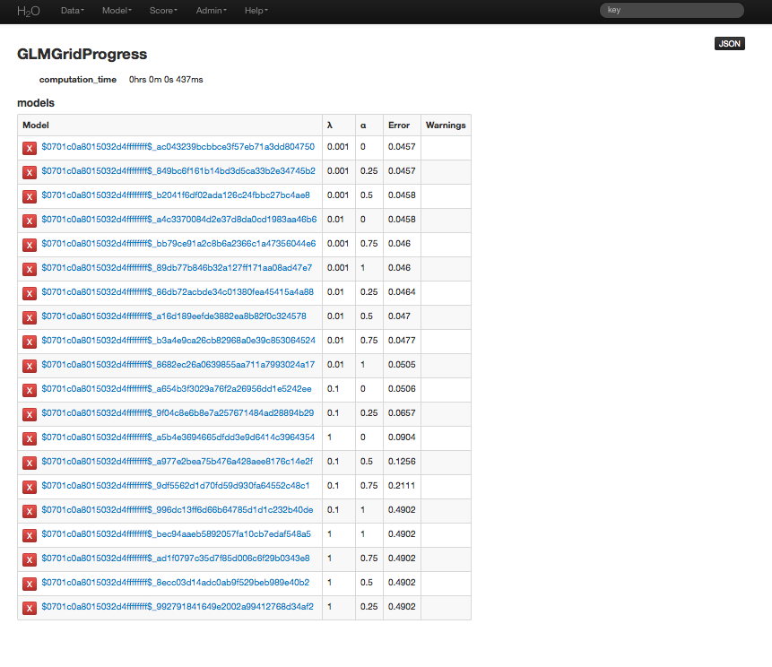
Individual model results
Validating on Testing Set
Models can be applied to holdout testing sets or prediction data, provided that the data are in the same format as the data originally used to generate the GLM model.
Note: If the models used for prediction have lambda search enabled, ~100 submodels are generated. To score a specific lambda value, select a lambda from the lambda row in the “Parameters” table at the top of the page. By default, H2O selects the “best” lambda value, which appears in bold in the lambda row in the “Parameters” table.
If you select a different lambda value, the page refreshes and the selected lambda appears in bold. If you click the Predict! link at the top of the page, the selected lambda is used for the prediction. However, if you select Score > Predict, the default “best” lambda value is used, not the selected value. To store the selected lambda value as the “best” value, click the Set lambda_value to current value! link.
- Click the Predict! link at the top of the GLM results page, or go to the drop-down Score menu and select Predict.
- If you clicked the Predict! link on the GLM results page, the model .hex key is entered automatically. Otherwise, enter the model .hex key in the “model” field.
- In the “data” field, enter the .hex key of the test data set and click Submit.
- For regression models, click the Score menu and select Confusion Matrix. For binomial models, click the Score menu and select AUC.
- In the “actual” field, enter the .hex key for the test data set.
- From the drop-down “vactual” list, select the column to use for prediction.
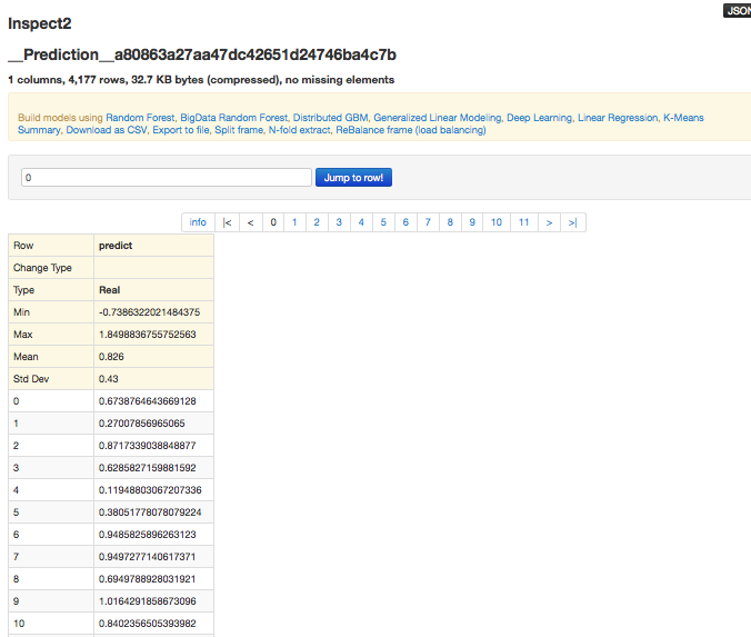
- In the “predict” field, enter the .hex key for the prediction generated in the first step.
- From the drop-down “vpredict” list, select predict.
- Click Submit.