Random Forest (RF)
RF is a powerful classification tool. When given a set of data, RF generates a forest of classification trees, rather than a single classification tree. Each of these trees generates a classification for a given set of attributes. The classification from each H2Otree can be thought of as a vote; the most votes determines the classification.
When to use RF
RF is a good choice when your objective is classification. For example:
“Given a large set of observations and attributes, the goal is to classify observations by spending habits.”
Defining a Model
Response Variable:
The variable on which you would like to classify
N Tree:
The number of trees the user would like to generate for classification
Features:
A user defined tuning parameter for controlling model complexity (by number of nodes); the number of features on which the trees are to split. In practice features is bounded between 1 and the total number of features in the data. In different fields features may also be called attributes or traits.
Depth:
A user defined tuning parameter for controlling model complexity (by number of edges); depth is the longest path from root to the furthest leaf.
- Stat type:
A choice of criteria that determines the optimum split at each node.
- Entropy:
- This is also known as information gain, entropy is a measure of uncertainty in a classification scheme. For example, if a two class population is 90% class A, and 10% class B, then there is a .90 probability that a randomly selected member of the population is A. This scheme has lower entropy than a population where 50% is class A, and 50% is class B. the objective of using the entropy impurity measure is to minimize this uncertainty.
- Gini:
- An impurity measure based on the disparities in attribute correlation between the most and least dominant classes in a node. The objective of using this impurity measure is to choose the feature split that best isolates the dominant class.
Ignore:
Is the set of columns other than the response variable that should be omitted from building the tree.
Sampling Strategy:
This allows the user to define whether or not the model needs to correct for unbalanced data by changing the mechanism through which training samples are generated.
Serves a similar purpose as class weights; It ensures that in unbalanced data the sample split for testing and training (used to calculate the out of bag error) every class is represented at least once. This insures that every class is included in the model, rather than being omitted by chance.
Random Sampling:
Samples subsets on which trees are built such that every observation has an equal chance of being drawn.
- Stratified Sampling:
- Partitions data set by classification before sampling, and then samples from each subset. This insures that each class will be represented in every split, even if the class being drawn in a random sample was a low probability event. It guarantees that when data are unbalanced, no class is omitted from the model by chance.
Sample:
User defined percentage of the observations in the data set to sample for the building of each tree.
Out of Bag Error Estimate:
Every tree RF internally constructs a test/ train split. The Kth tree is built by pulling a sample on the data set, bootstrapping, and using the result to build a tree. Observations not used to build the tree are then run down the tree to see what classification they are assigned. The OOB error rate is calculated by calculating the error rate for each class and then averaging over all classes.Bin Limit:
A user defined tuning parameter for controlling model complexity, bin limit caps the the maximum number of groups into which the orginal data are to be categorized.Seed:
A large number that allows the analyst to recreate an analysis by specifying a starting point for black box processes that would otherwise occur at a randomly chosen place within the data.Class Weight:
When observed classifications in training data are uneven, users may wish to correct this by weighting. Weights should be assigned so that if chosen at random, an observation of each classification has an equal chance. For example, if there are two classifications A and B in a data set, such that As occur about 10% of the time, and Bs occur the rest, A should given a weight of 5, and B of .56.
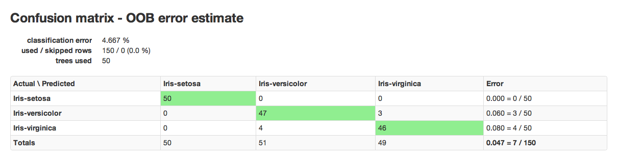
Interpreting Results
RF results are comprised of a model key and a confusion matrix. The model key specifies the full forest of trees to be used for predicting classifications.
An example of a confusion matrix is given below:
The highlighted fields across the diagonal indicate the number the number of true members of the class who were correctly predicted as true. In this case, of 111 total members of class F, 44 were correctly identified as class F, while a total of 80 observations were incorrectly classified as M or I, yielding an error rate of 0.654.
In the column for class F, 11 members of I were incorrectly classified as F, 56 as male, and a total of 111 observations in the set were identified as F.
The overall error rate is shown in the bottom right field. It reflects the total number of incorrect predictions divided by the total number of rows.
RF Error Rates
H2O’s Random Forest Algo produces a dynamic confusion matrix. As each tree is built and OOBE (out of bag error estimate) is recalculated, expected behavior is that error rate increases before it decreases. This is a natural outcome of Random Forest’s learning process. When there are only a few trees, built on random subsets, the error rate is expected to be relatively high. As more trees are added, and thus more trees are “voting” for the correct classification of the OOB data, the error rate should decrease.