Random Forest Tutorial
The purpose of this tutorial is to walk the new user through a Random Forest analysis beginning to end. By the end of this tutorial the user should know how to specify, run, and interpret Random Forest.
Those who have never used H2O before should see the quick start guide for how to run H2O on your computer.
Getting Started
This tutorial uses a publicly available data set that can be found
Internet ads data set http://archive.ics.uci.edu/ml/machine-learning-databases/internet_ads/
The data are composed of 3279 observations, 1557 attributes, and an priori grouping assignment. The objective is to build a prediction tool that predicts whether an object is an internet ad or not.
- Under the drop down menu Data select Upload and use the helper to upload data.
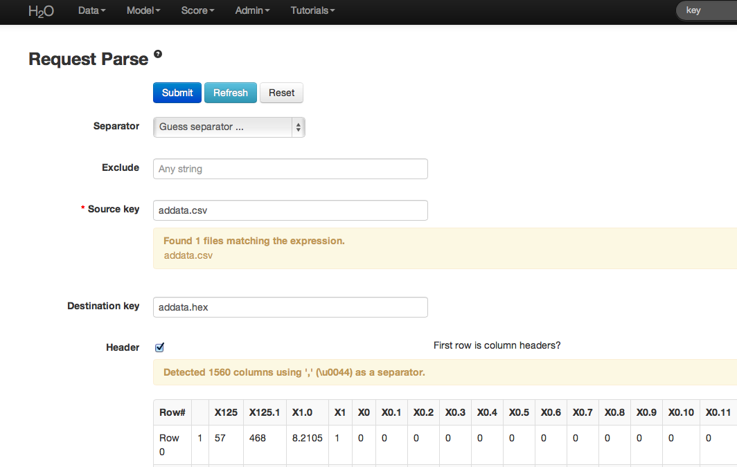
- After uploading page is redirected to a page with the header “Request Parse”. Select whether the first row of the data set is a header as appropriate. All settings can be left in default. Press Submit.
- Parsing data into H2O generates a .hex key (“data name.hex”).
Building a Model
- Once data are parsed a horizontal menu will appear at the top of the screen reading “Build model using ... ”. Select Random Forest here, or go to the drop down menu “Model” and find Random Forest there.
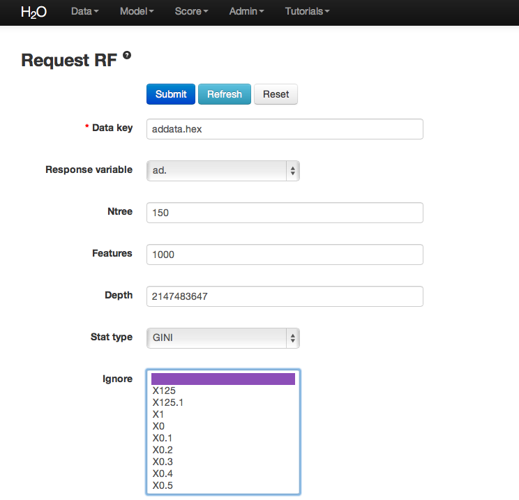
- In the field for Data Key enter the .hex key generated when data were parsed.
- In Ntree specify the number of trees to be built; in this case 150.
- Features specifies the number of features on which the trees will split. For this analysis specify Features to be 1000.
- Depth specifies the maximum distance from root to terminal node. Leave this in default.
- Stat type provides a choice between split criteria. Entropy maximizes information gain, where Gini seeks to isolate the dominant category at each node. Choose Gini for this analysis.
- Ignore provides a list of attributes. Selecting an attribute will exclude it from consideration in tree building.
- Class weights and sampling strategy are both used to correct for unbalanced data. Leave both in default here.
- Sample specifies the proportion of observations sampled when building any given tree. The observations omitted from building a tree are run down the tree, and the classification error rate of that tree is estimated using the error rate from this holdout set.
- Exclusive split limit defines the minimum number of objects to be grouped together in any terminal node.
RF Output
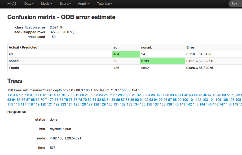
The RF output of main interest is a confusion matrix detailing the classification error rates for each level in the range of the target variable. In addition to the confusion matrix, the overall classification error, the number of trees and data use descriptives are included.
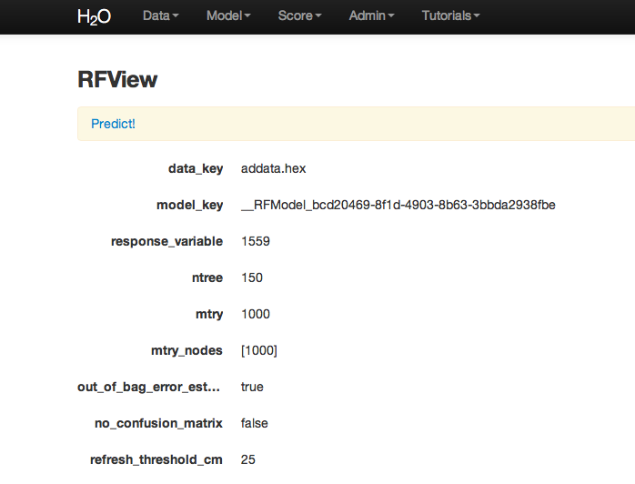
RF inspect in total also includes information about the user chosen tuning parameters at the top of RFView. At the top of the page there is also an option to go directly to generating predictions for another dataset.
RF Predict
To generate a prediction click on the Predict! link at the top of the RFView page. This function can also be found by going to the drop down menu Score, and choosing predict.
Using the predict function requires the .hex key associated with a model. To find this go to the drop down menu Admin and select Jobs.
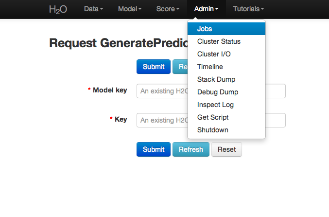
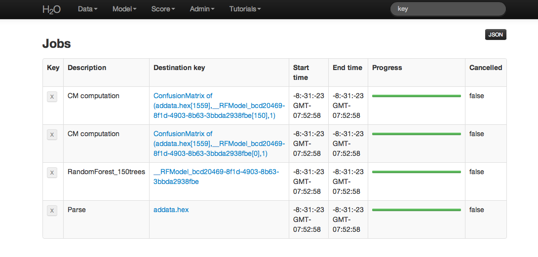
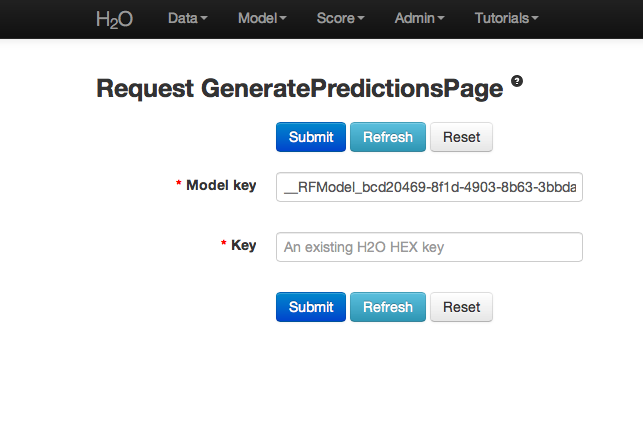
All jobs created in the current instance of H2O will be listed here. Find the appropriate job (here labeled “Random Forest 150 Trees”). Save the associated key to clipboard, and paste into the model key field in the Request Generate Predictions Page. Enter a .hex key associated with a parsed data set other than the one used to build the model.
THE END.